

A Sparse-Reconstruction-Based Fast Localization Algorithm for Mixed Far-Field and Near-Field Sources
-
摘要: 协方差向量具有比原始阵列输出更高的信噪比增益,该文将远近场混合源模型扩展到协方差域,并针对稀疏重构远近场混合源定位算法时间复杂度高的问题,提出了一种基于协方差域阵列信号模型和广义近似消息传递(GAMP)-变分贝叶斯推断(VBI)的远近场混合源定位改进算法(FN-GAMP-CVBI),实现了计算效率与定位精度的有效平衡。数值仿真表明,与现有的远近场混合源定位算法相比,该文所提算法具有更高的远近场源定位精度和较低的计算时间。湖试数据结果进一步验证了该文所提算法的高效性和有效性。Abstract:
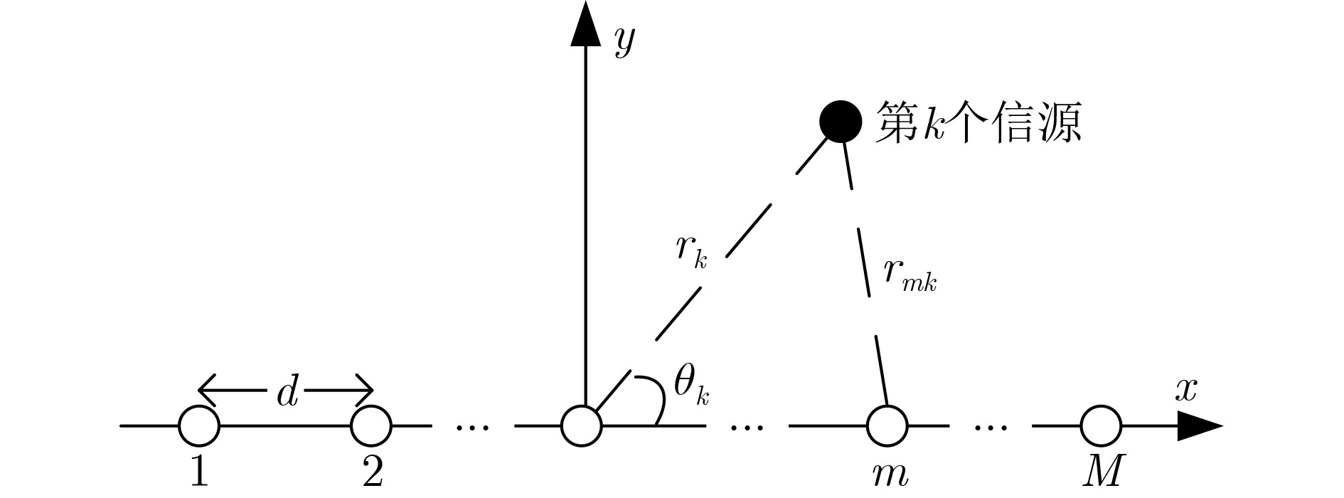
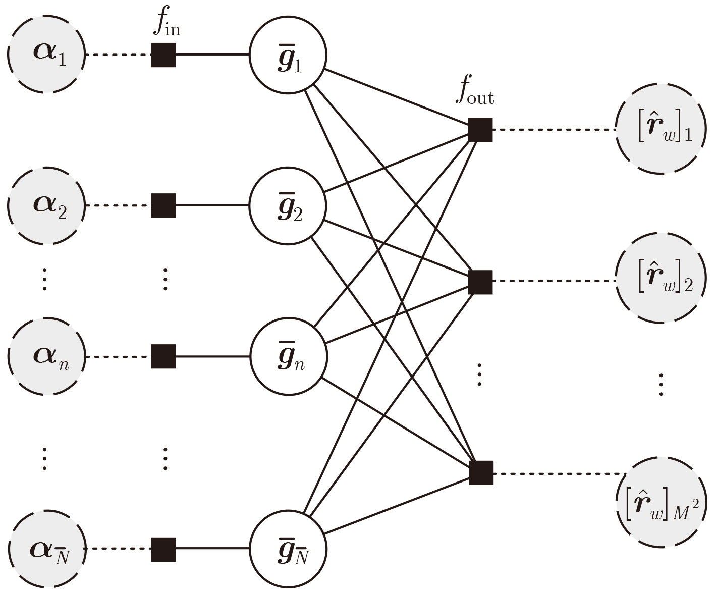
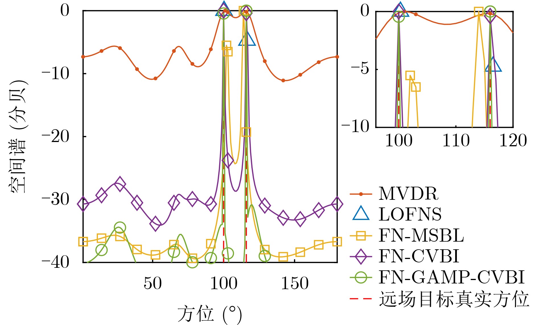
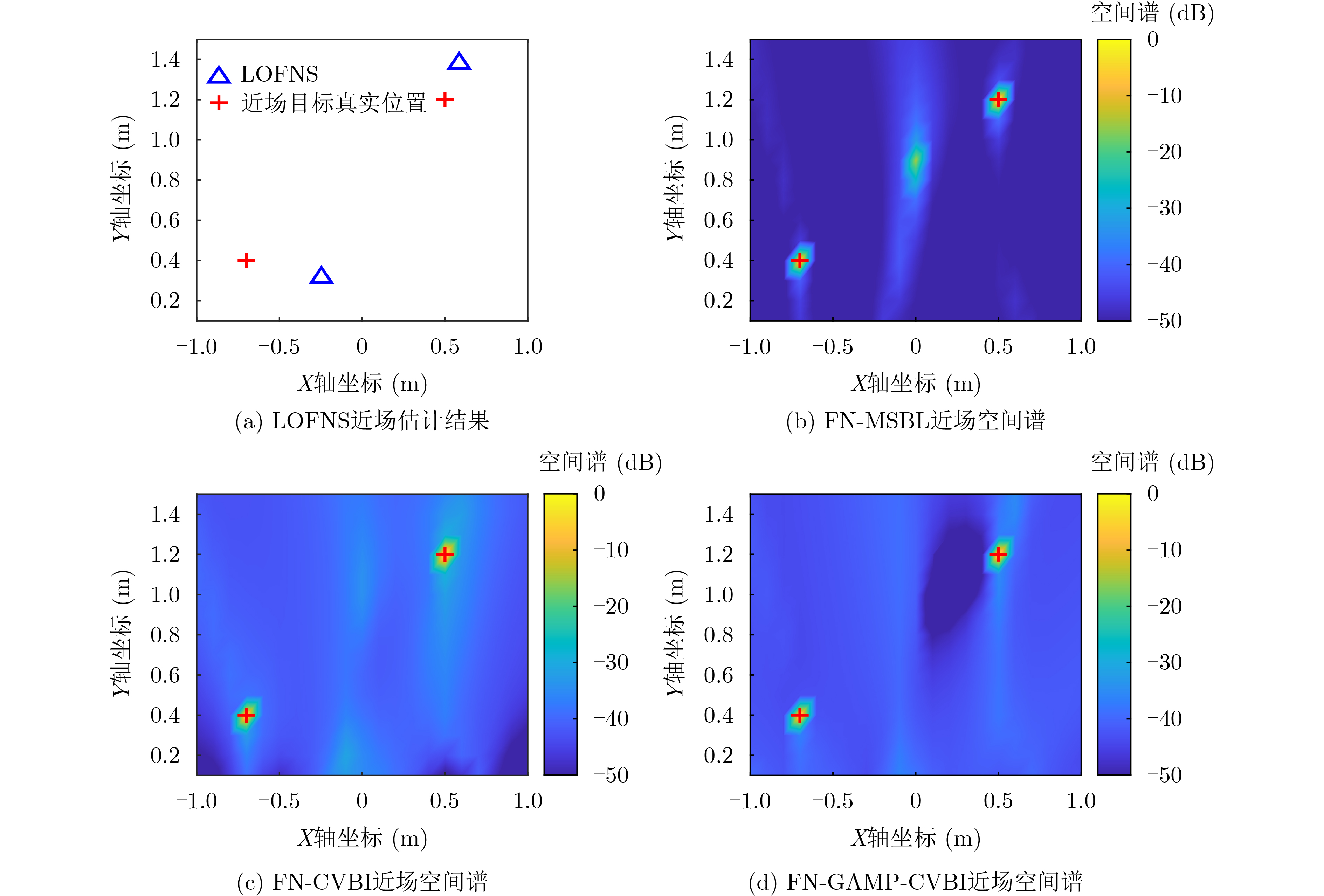
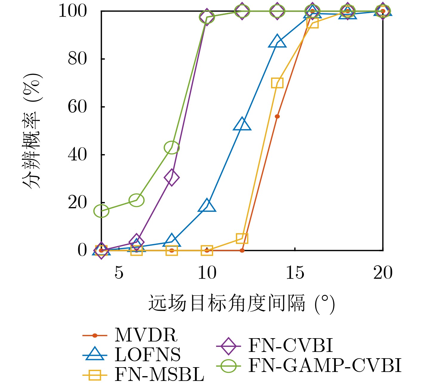
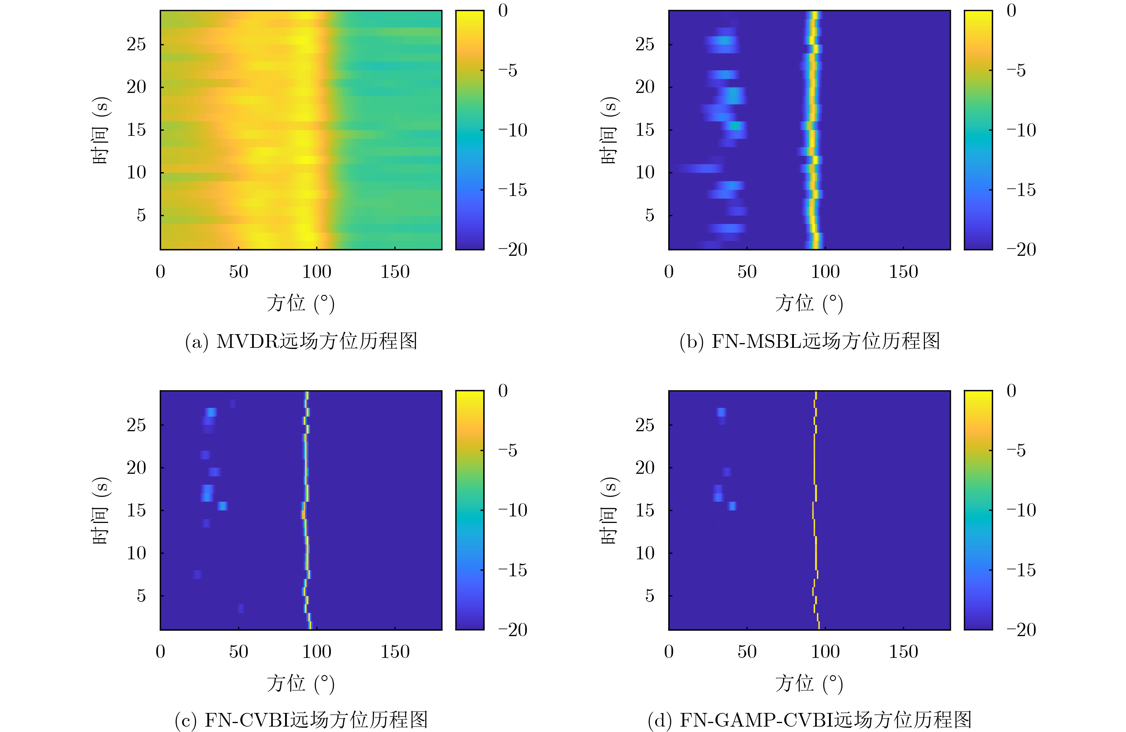
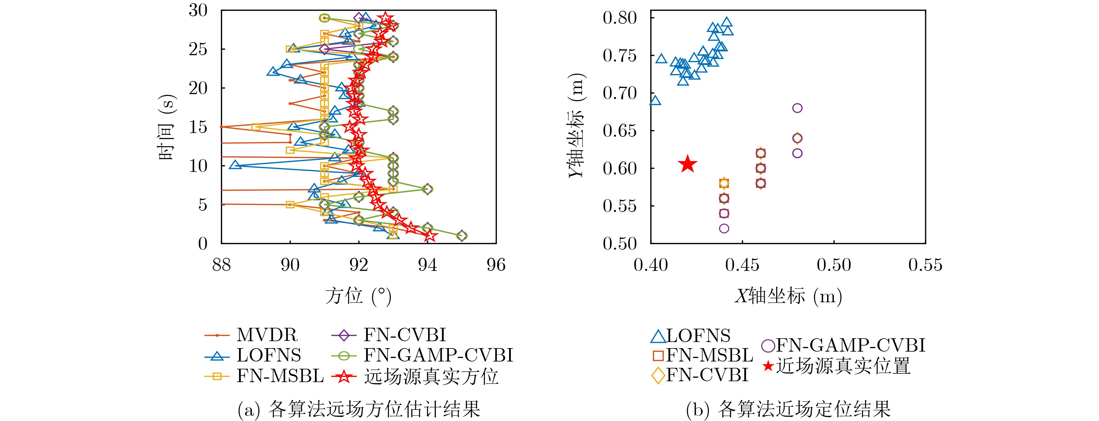
Objective Source localization is a key research topic in array signal processing, with applications in radar, sonar, and wireless communications. Conventional localization methods based solely on far-field or near-field models face clear limitations when separating and localizing mixed far-field and near-field sources. Existing approaches, such as subspace-based methods, often show high computational complexity, limited localization accuracy, and degraded performance under low Signal-to-Noise Ratio (SNR) conditions. In addition, many methods assume that near-field sources lie strictly within the Fresnel region, which leads to localization errors and a reduced effective array aperture. Improved algorithms, such as Multiple Sparse Bayesian Learning for Far- and Near-Field Sources (FN-MSBL), overcome part of these limitations and achieve higher localization accuracy. However, their reliance on iterative matrix inversion leads to high computational cost and restricts real-time applicability. Therefore, this study aims to address these issues by proposing a novel algorithm that develops a sparse representation model for mixed far-field and near-field sources in the covariance domain and integrates sparse reconstruction with the Generalized Approximate Message Passing (GAMP) and Variational Bayesian Inference (VBI) frameworks. The objective is to achieve high-precision localization of mixed sources while substantially reducing computational cost. Methods Two algorithms, termed Covariance-Based VBI for Far- and Near-Field Sources (FN-CVBI) and Covariance-Based GAMP-VBI for Far- and Near-Field Sources (FN-GAMP-CVBI), are developed. First, a unified sparse representation model for mixed far-field and near-field sources is constructed based on the covariance vector. This representation benefits from the improved SNR of the covariance vector relative to the original array output, which improves far-field Direction of Arrival (DOA) estimation. Second, to reduce estimation errors in the sample covariance matrix, a pre-whitening operation is applied to the covariance vector to minimize inter-element correlation and improve robustness. Third, a hierarchical Bayesian model is established to impose sparsity, and VBI is employed to estimate model parameters through iterative posterior updates. Fourth, to reduce the computational burden associated with conventional VBI, GAMP is embedded into the VBI framework to replace matrix inversion operations. The detailed implementation of GAMP is given in Algirithm1 . By combining sparse reconstruction, VBI, and GAMP, the proposed approach improves localization accuracy while markedly reducing computational complexity.Results and Discussions The proposed FN-GAMP-CVBI algorithm shows clear improvements in both localization accuracy and computational efficiency. Complexity analysis indicates a substantial reduction in computational cost ( Table 1 ). In terms of localization performance, FN-CVBI and FN-GAMP-CVBI outperform comparative methods, including LOFNS and FN-MSBL (Fig. 3 ,Fig. 4 ), particularly under low SNR conditions and with sufficient snapshots (Fig. 5 ,Fig. 6 ). The proposed methods also show strong capability in resolving closely spaced far-field sources (Fig. 7 ). Experimental validation using lake trial data confirms these findings, as reflected by sharper spectral peaks and fewer false peaks in the background noise of the Bearing Time Recording (BTR) results (Fig. 9 ). FN-CVBI achieves the highest accuracy in far-field DOA estimation and near-field localization. The computational time of FN-GAMP-CVBI is reduced by up to 95% compared with FN-MSBL (Table 3 ), demonstrating its suitability for real-time applications.Conclusions A sparse-reconstruction-based approach for mixed far-field and near-field source localization is presented by integrating sparse reconstruction with the GAMP-VBI framework. The proposed FN-GAMP-CVBI algorithm addresses the limitations of existing methods and achieves a balanced trade-off between localization accuracy and computational efficiency. Simulation results confirm superior performance, especially under low SNR conditions with sufficient snapshots, and experimental results further support the effectiveness of the approach. The low computational complexity and ability to handle mixed-source scenarios indicate that the proposed algorithm is well suited for real-time localization in complex environments. -
1 基于GAMP计算近似后验的算法流程
输入:参数估计${\boldsymbol{\alpha}} $, ${\beta _0}$,协方差向量${\hat {\boldsymbol{r}}_w}$,过完备字典$ {\bar{\boldsymbol{\varPhi}} _w} $。 (1) 初始化:$l = 1$,${\hat {\boldsymbol{g}}^{(0)}} = {{{\textit{0}}}}$,${{\boldsymbol{s}}^{(0)}} = {{{\textit{0}}}}$,${\boldsymbol{S}} = {\left| {{{\bar {\boldsymbol{\varPhi}} }_w}} \right|^2}$,${\boldsymbol{\tau}} _g^{(0)} = {{\boldsymbol{\alpha}} ^{ - 1}}$。 (2) 循环执行如下步骤 (a) 输出线性步骤 $\left.\begin{gathered} {\boldsymbol{\tau}} _p^{(l)} = {\boldsymbol{S\tau}} _g^{(l - 1)} \\ {\boldsymbol{\mu}} _p^{(l)} = {{\bar {\boldsymbol{\varPhi}} }_w}{{\hat {\boldsymbol{g}}}^{(l - 1)}} - {\boldsymbol{\tau}} _p^{(l)} \circ {{\boldsymbol{s}}^{(l - 1)}} \\ \end{gathered}\right\} $ (25) (b) 输出非线性步骤 $ \left.\begin{gathered}\boldsymbol{s}^{(l)}=\left(1-\lambda_g\right)\boldsymbol{s}^{(l-1)}+\lambda_g\boldsymbol{\mathit{g}}_{\mathrm{out}}\left(\hat{\boldsymbol{r}}_w,\boldsymbol{\mu}_p^{(l)},\boldsymbol{\tau}_p^{(l)},\beta_0\right) \\ \boldsymbol{\tau}_s^{(l)}=-g'_{\mathrm{out}}\left(\hat{\boldsymbol{r}}_w,\boldsymbol{\mu}_p^{(l)},\boldsymbol{\tau}_p^{(l)},\boldsymbol{\mathit{\beta}}_0\right)\end{gathered}\right\} $ (26) (c) 输入线性步骤 $ \left.\begin{gathered} {\boldsymbol{\tau}} _q^{(l)} = {{\boldsymbol{1}} \mathord{\left/ {\vphantom {1 {{S^{\rm T}}\tau _s^{(l)}}}} \right. } {{{\boldsymbol{S}}^{\rm T}}{\boldsymbol{\tau}} _s^{(l)}}} \\ {\boldsymbol{\mu}} _q^{(l)} = {{\hat {\boldsymbol{g}}}^{(l - 1)}} + {\boldsymbol{\tau }}_q^{(l)} \circ \left( {{{\bar {\boldsymbol{\varPhi}} }_w}^{\rm H}{{\boldsymbol{s}}^{(l)}}} \right) \end{gathered}\right\} $ (27) (d) 输入非线性步骤 $ \left.\begin{gathered} {{\hat {\boldsymbol{g}}}^{(l)}} = \left( {1 - {\lambda _g}} \right){{\hat {\boldsymbol{g}}}^{(l - 1)}} + {\lambda _g}{g_{{\mathrm{in}}}}({\boldsymbol{\mu}} _q^{(l)},{\boldsymbol{\tau}} _q^{(l)},{\boldsymbol{\alpha}} ) \\ {\boldsymbol{\tau}} _g^{(l)} = {\boldsymbol{\tau}} _q^{(l)} \circ {{g'}_{{\mathrm{in}}}}({\boldsymbol{\mu}} _q^{(l)},{\boldsymbol{\tau}} _q^{(l)},{\boldsymbol{\alpha}} ) \end{gathered}\right\} $ (28) (e)令$l = l + 1$,循环执行(a)到(e)步直到迭代次数$l$和容差$ \xi= \left\| \hat{\boldsymbol{g}}^{(l)}-\hat{\boldsymbol{g}}^{(l-1)} \right\| _2\mathord{\left/\vphantom{ \left\| \hat{g}^{(l)}-\hat{g}^{(l-1)} \right\| _2 \left\| \hat{g}^{(l)} \right\| }\right.} \left\| \hat{\boldsymbol{g}}^{(l)} \right\| _2 $满足条件$l \ge {G_l}$或$\xi \le {G_\zeta }$时停止迭代,其中${G_l}$为设定最大GAMP迭代次数,${G_\zeta }$为设定的容差门限。 (3) 输出:$ \boldsymbol{\overline{g}} $的近似后验分布的估计结果$ q(\bar {\boldsymbol{g}}) = \mathcal{C}\mathcal{N}(\hat {\boldsymbol{\mu}} ,\hat {\boldsymbol{\varSigma}} ) $,其均值和方差为 $ \left. \begin{gathered} \hat {\boldsymbol{\mu}} = {{\hat {\boldsymbol{g}}}^{(l)}} \\ \hat {\boldsymbol{\varSigma}} = {\mathrm{diag}}\left\{ {{\boldsymbol{\tau}} _g^{(l)}} \right\} \\ \end{gathered} \right\} $ (29)  下载: 导出CSV
表 1 各算法的单次迭代时间复杂度
算法 时间复杂度 FN-MSBL $O\left( {\left( {\bar N - 1} \right)\left( {{M^2} + MT} \right) + {{\left( {\bar N - 1} \right)}^2}M + {M^3} + {M^2}T} \right)$ FN-CVBI $ O\left( {\max \left\{ {{{\bar N}^3} + {{\bar N}^2}{M^2},\bar N{M^4} + {{\bar N}^2}{M^2} + {M^6}} \right\}} \right) $ FN-GAMP-CVBI $O\left( {\bar N{M^2}} \right)$
下载: 导出CSV
表 3 各算法远近场混合源定位结果的统计对比
算法 远场RMSE
(°)近场RMSE
(m)平均计算时间
(ms)LOFNS 1.427 0.139 0.240 FN-MSBL 1.374 0.046 3.784 FN-CVBI 0.804 0.045 3.828 FN-GAMP-CVBI 0.819 0.049 0.184
下载: 导出CSV
-
[1] LIANG Guolong, CHEN Yu, WANG Jinjin, et al. Enhanced noise resilience in passive tone detection via broad-receptive field complex-valued convolutional neural networks[J]. The Journal of the Acoustical Society of America, 2024, 155(6): 3968–3982. doi: 10.1121/10.0026438. [2] DU Zhiyao, HAO Yu, QIU Longhao, et al. Sparsity-based direction-of-arrival estimation in the presence of near-field and far-field interferences for small-scale platform sonar arrays[J]. The Journal of the Acoustical Society of America, 2024, 156(5): 2989–3005. doi: 10.1121/10.0034240. [3] LEE J H, CHEN Y M, and YEH C C. A covariance approximation method for near-field direction-finding using a uniform linear array[J]. IEEE Transactions on Signal Processing, 1995, 43(5): 1293–1298. doi: 10.1109/78.382421. [4] LIANG Junli and LIU Ding. Passive localization of mixed near-field and far-field sources using two-stage MUSIC algorithm[J]. IEEE Transactions on Signal Processing, 2010, 58(1): 108–120. doi: 10.1109/TSP.2009.2029723. [5] HE Jin, SWAMY M N S, and AHMAD M O. Efficient application of MUSIC algorithm under the coexistence of far-field and near-field sources[J]. IEEE Transactions on Signal Processing, 2012, 60(4): 2066–2070. doi: 10.1109/TSP.2011.2180902. [6] ZUO Weiliang, XIN Jingmin, ZHENG Nanning, et al. Subspace-based localization of far-field and near-field signals without eigendecomposition[J]. IEEE Transactions on Signal Processing, 2018, 66(17): 4461–4476. doi: 10.1109/tsp.2018.2853124. [7] LI Chenmu, LIANG Guolong, QIU Longhao, et al. An efficient sparse method for direction-of-arrival estimation in the presence of strong interference[J]. The Journal of the Acoustical Society of America, 2023, 153(2): 1257–1271. doi: 10.1121/10.0017256. [8] WANG Bo, LIU Juanjuan, and SUN Xiaoying. Mixed sources localization based on sparse signal reconstruction[J]. IEEE Signal Processing Letters, 2012, 19(8): 487–490. doi: 10.1109/lsp.2012.2204248. [9] CHEN Mengya, LIN Wei, ZHAO Yongwei, et al. Gridless mixed-field sources localisation algorithm based on covariance matrix reconstruction[J]. Journal of Physics: Conference Series, 2024, 2849: 012117. doi: 10.1088/1742-6596/2849/1/012117. [10] QI Meibin, REN Weijie, and XIANG Houhong. Separation of mixed near-field and far-field sources and DOA estimation based on deep learning[C]. ICAIT 2023 - 2023 IEEE 15th International Conference on Advanced Infocomm Technology, Hefei, China, 2023: 226–233. doi: 10.1109/ICAIT59485.2023.10367306. [11] LIANG Guolong, ZHAO Benbin, and FAN Zhan. Direction of arrival estimation under near-field interference using matrix filter[J]. Journal of Computational Acoustics, 2015, 23(4): 1540007. doi: 10.1142/S0218396X1540007X. [12] HAWKES M and NEHORAI A. Acoustic vector-sensor correlations in ambient noise[J]. IEEE Journal of Oceanic Engineering, 2001, 26(3): 337–347. doi: 10.1109/48.946508. [13] 邱龙皓, 梁国龙, 王燕, 等. 稀疏贝叶斯学习远近场混合源定位方法[J]. 声学学报, 2018, 43(1): 1–11. doi: 10.15949/j.cnki.0371-0025.2018.01.001.QIU Longhao, LIANG Guolong, WANG Yan, et al. Mixed near-field and far-field sources localization method using sparse Bayesian learning[J]. Acta Acustica, 2018, 43(1): 1–11. doi: 10.15949/j.cnki.0371-0025.2018.01.001. [14] 刘章孟. 基于信号空域稀疏性的阵列处理理论与方法[D]. [博士论文], 国防科学技术大学, 2012.LIU Zhangmeng. Spatial sparsity-based theory and methodsof array signal processing[D]. [Ph. D. dissertation], National University of Defense Technology, 2012. [15] AL-SHOUKAIRI M, SCHNITER P, and RAO B D. A GAMP-based low complexity sparse bayesian learning algorithm[J]. IEEE Transactions on Signal Processing, 2018, 66(2): 294–308. doi: 10.1109/TSP.2017.2764855. [16] LI Ninghui, ZHANG Xiaokuan, ZONG Binfeng, et al. An off-grid direction-of-arrival estimator based on sparse Bayesian learning with three-stage hierarchical Laplace priors[J]. Signal Processing, 2024, 218: 109371. doi: 10.1016/j.sigpro.2023.109371. [17] TIPPING M E. Sparse Bayesian learning and the relevance vector machine[J]. The Journal of Machine Learning Research, 2001, 1: 211–244. doi: 10.1162/15324430152748236. [18] TZIKAS D G, LIKAS A C, and GALATSANOS N P. The variational approximation for Bayesian inference[J]. IEEE Signal Processing Magazine, 2008, 25(6): 131–146. doi: 10.1109/msp.2008.929620. [19] RANGAN S. Generalized approximate message passing for estimation with random linear mixing[C]. IEEE International Symposium on Information Theory, St. Petersburg, Russia, 2011: 2168–2172. doi: 10.1109/ISIT.2011.6033942. -

 下载:
下载:


图(10) / 表(4)
计量
- 文章访问数: 620
- HTML全文浏览量: 299
- PDF下载量: 55
- 被引次数: 0
