

Unbiased Self-synchronous Scrambler Identification Based on Log Conditional Likelihood Ratio
-
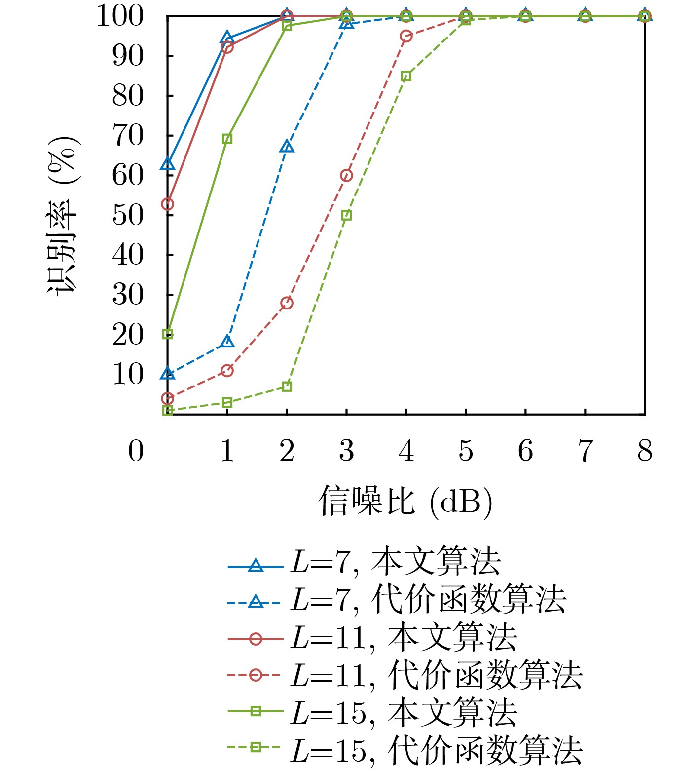
摘要: 为克服现有无偏自同步扰码识别算法在低信噪比(SNR)下存在适应性差的缺点,该文提出一种基于对数条件似然比的软判决识别方法。该方法首先构建了线性分组码自同步加扰和卷积码自同步加扰的对偶向量积线性约束方程;然后推导了基于软判决的对数条件似然比函数衡量方程的成立概率,并分析了其均值和方差的分布特性;最后通过2元假设和推导的相应判别门限来完成两种自同步加扰的识别。仿真结果表明,所提算法能够在低信噪比下完成生成多项式的识别,具有较好的适应能力,与基于求解代价函数的识别方法相比,在信噪比低于3 dB时的算法识别率得到较大提高,识别率为90%时,约有3 dB的性能增益。Abstract: To overcome the drawback of poor adaptability of existing unbiased self-synchronous scrambling code recognition algorithms at low Signal-to-Noise Ratios (SNR), a soft-judgement recognition method based on the log conditional likelihood ratio is proposed. Firstly, the linear constraint equations for the pairwise even-vector product of the self-synchronous scrambler of linear grouping codes and the self-synchronous scrambler of convolutional codes are constructed, and then the log likelihood ratio function is introduced, the log conditional likelihood ratio function based on the soft judgment is constructed, and the distribution characteristics of its mean and variance are analyzed. Finally the identification of self-synchronous scrambler of linear grouping codes and self-synchronous scrambler of convolutional codes is accomplished through binary assumption and the derived coresponding judgement threshold value. The simulations show that the proposed algorithm is able to complete the recognition of generating polynomials at low signal-to-noise ratios, and has a good low signal-to-noise adaptation capability. Compared with the recognition method based on solving the cost function, the recognition rate of the algorithm is greatly improved at signal-to-noise ratios below 3 dB, and when the recognition rate is 90%, the proposed algorithm achieves a performance gain of about 3 dB.
-
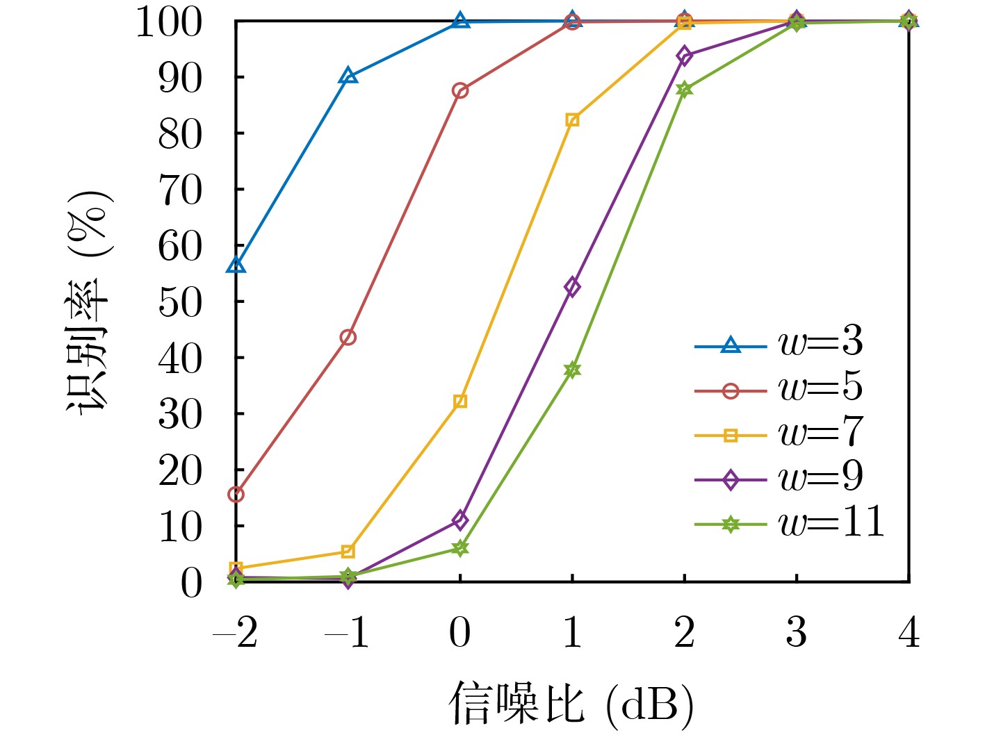
表 1 卷积码参数设定(不同码重)
码重$w$ 生成多项式 3 [$1,1 + {D^5}$] 5 [$1 + {D^5},1 + {D^4} + {D^5}$] 7 [$1 + {D^3} + {D^5},1 + {D^3} + {D^4} + {D^5}$] 9 [$1 + {D^2} + {D^4} + {D^5},1 + {D^2} + {D^3} + {D^4} + {D^5}$] 11 [$1 + D + {D^3} + {D^4} + {D^5},1 + D + {D^2} + {D^3} + {D^4} + {D^5}$]  下载: 导出CSV
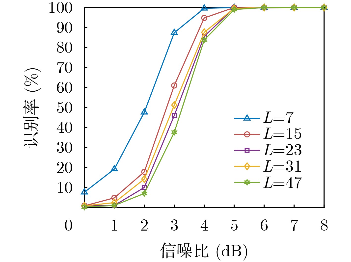
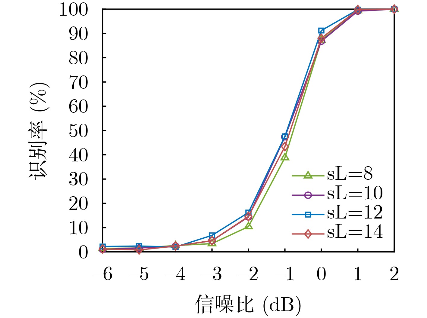
表 2 卷积码参数设定(不同编码约束长度)
编码约束长度${\text{sL}}$ 生成多项式 8 [$1 + {D^3},1 + {D^2} + {D^3}$] 10 [$1 + {D^4},1 + {D^3} + {D^4}$] 12 [$1 + {D^5},1 + {D^4} + {D^5}$] 14 [$1 + D,1 + D + {D^6}$]
下载: 导出CSV
-
[1] 刘玉君. 信道编码[M]. 郑州: 河南科学技术出版社, 2006: 51–52.LIU Yujun. Channel coding[M]. Zhengzhou: Henan Science and Technology Press, 2006: 51–52. [2] DING Yong, HUANG Zhiping, and ZHOU Jing. Joint blind reconstruction of the cyclic codes and self-synchronous scramblers in a noisy environment[J]. IEEE Transactions on Communications, 2023, 71(8): 4411–4424. doi: 10.1109/TCOMM.2023.3280214. [3] KIM D and YOON D. Blind estimation of self-synchronous scrambler in DSSS systems[J]. IEEE Access, 2021, 9: 76976–76982. doi: 10.1109/ACCESS.2021.3083071. [4] KIM Y, KIM J, SONG J, et al. Blind estimation of self-synchronous scrambler using orthogonal complement space in DSSS systems[J]. IEEE Access, 2022, 10: 66522–66528. doi: 10.1109/ACCESS.2022.3185066. [5] KIM D and YOON D. Novel algorithm for blind estimation of scramblers in DSSS systems[J]. IEEE Transactions on Information Forensics and Security, 2023, 18: 2292–2302. doi: 10.1109/TIFS.2023.3265345. [6] DING Yong, HUANG Zhiping, and ZHOU Jing. Joint blind reconstruction of cyclic codes and self-synchronous scramblers[J]. IET Communications, 2023, 17(13): 1478–1491. doi: 10.1049/cmu2.12636. [7] DING Yong, HUANG Zhiping, and ZHOU Jing. Fast reconstruction of feedback polynomials for synchronous scramblers in a noisy environment[J]. IET Communications, 2022, 16(19): 2293–2300. doi: 10.1049/cmu2.12482. [8] DING Yong, HUANG Zhiping, and ZHOU Jing. Blind identification of feedback polynomials for synchronous scramblers in a noisy environment[J]. IET Communications, 2023, 17(3): 296–305. doi: 10.1049/cmu2.12537. [9] CHOI J and YU N. Secure image encryption based on compressed sensing and scrambling for internet-of-multimedia things[J]. IEEE Access, 2022, 10: 10706–10718. doi: 10.1109/ACCESS.2022.3145005. [10] ZHENG Jieheng, ZHANG Lin, FENG Yan, et al. Blockchain-based key management and authentication scheme for IoT networks with chaotic scrambling[J]. IEEE Transactions on Network Science and Engineering, 2023, 10(1): 178–188. doi: 10.1109/TNSE.2022.3205913. [11] TAN Jiyuan, ZHANG Limin, and ZHONG Zhaogen. Distinction of scrambled linear block codes based on extraction of correlation features[J]. Applied Sciences, 2022, 12(21): 11305. doi: 10.3390/app122111305. [12] TAN Jiyuan, ZHANG Limin, and ZHONG Zhaogen. Reconstruction of a synchronous scrambler based on average check conformity[J]. Mathematical Problems in Engineering, 2022, 2022: 6318317. doi: 10.1155/2022/6318317. [13] 陈泽亮, 彭华, 巩克现, 等. 基于软信息的扰码盲识别方法[J]. 通信学报, 2017, 38(3): 174–182. doi: 10.11959/j.issn.1000-436x.2017043.CHEN Zeliang, PENG Hua, GONG Kexian, et al. Scrambler blind recognition method based on soft information[J]. Journal on Communications, 2017, 38(3): 174–182. doi: 10.11959/j.issn.1000-436x.2017043. [14] 张立民, 谭继远, 钟兆根, 等. 基于余弦符合度的自同步扰码盲识别[J]. 电子与信息学报, 2022, 44(4): 1412–1420. doi: 10.11999/JEIT210248.ZHANG Limin, TAN Jiyuan, ZHONG Zhaogen, et al. Blind recognition of self-synchronous scramblers based on cosine conformity[J]. Journal of Electronics & Information Technology, 2022, 44(4): 1412–1420. doi: 10.11999/JEIT 210248. [15] 张旻, 吕全通, 朱宇轩. 基于线性分组码的自同步扰码盲识别[J]. 应用科学学报, 2015, 33(2): 178–186. doi: 10.3969/j.issn.0255-8297.2015.02.007.ZHANG Min, LV Quantong, and ZHU Yuxuan. Blind recognition of self-synchronized scrambler based on linear block code[J]. Journal of Applied Sciences, 2015, 33(2): 178–186. doi: 10.3969/j.issn.0255-8297.2015.02.007. [16] 吕全通, 张旻, 李歆昊, 等. 基于码重分布距离的自同步扰码识别方法[J]. 探测与控制学报, 2015, 37(5): 7–13.LV Quantong, ZHANG Min, LI Xinhao, et al. Self-synchronized scrambler recognition based on code weight distributing distance[J]. Journal of Detection & Control, 2015, 37(5): 7–13. [17] 尹瑾, 王建新. RS码的自同步扰码盲识别方法[J]. 计算机工程与应用, 2017, 53(22): 77–81,86. doi: 10.3778/j.issn.1002-8331.1605-0357.YIN Jin and WANG Jianxin. Blind recognition method of self-synchronized scrambler after the Reed-Solomon code[J]. Computer Engineering and Applications, 2017, 53(22): 77–81,86. doi: 10.3778/j.issn.1002-8331.1605-0357. [18] 张天骐, 易琛, 张刚, 等. 基于高斯列消元法的线性分组码参数盲识别[J]. 系统工程与电子技术, 2013, 35(7): 1514–1519. doi: 10.3969/j.issn.1001-506X.2013.07.27.ZHANG Tianqi, YI Chen, ZHANG Gang, et al. Blind identification of parameters of linear block codes based on columns Gaussian elimination[J]. Systems Engineering and Electronics, 2013, 35(7): 1514–1519. doi: 10.3969/j.issn.1001-506X.2013.07.27. [19] 韩树楠, 张旻, 李歆昊. 基于构造代价函数求解的自同步扰码盲识别方法[J]. 电子与信息学报, 2018, 40(8): 1971–1977. doi: 10.11999/JEIT171026.HAN Shunan, ZHANG Min, and LI Xinhao. A blind identification method of self-synchronous scramblers based on optimization of established cost function[J]. Journal of Electronics & Information Technology, 2018, 40(8): 1971–1977. doi: 10.11999/JEIT171026. [20] HAGENAUER J, OFFER E, and PAPKE L. Iterative decoding of binary block and convolutional codes[J]. IEEE Transactions on Information Theory, 1996, 42(2): 429–445. doi: 10.1109/18.485714. -

 下载:
下载:


图(9) / 表(2)
计量
- 文章访问数: 710
- HTML全文浏览量: 441
- PDF下载量: 47
- 被引次数: 0
