认知车联网中评估频谱稳定性的动态频谱接入算法

马彬; 杨祖敏; 谢显中

doi:10.11999/JEIT240927

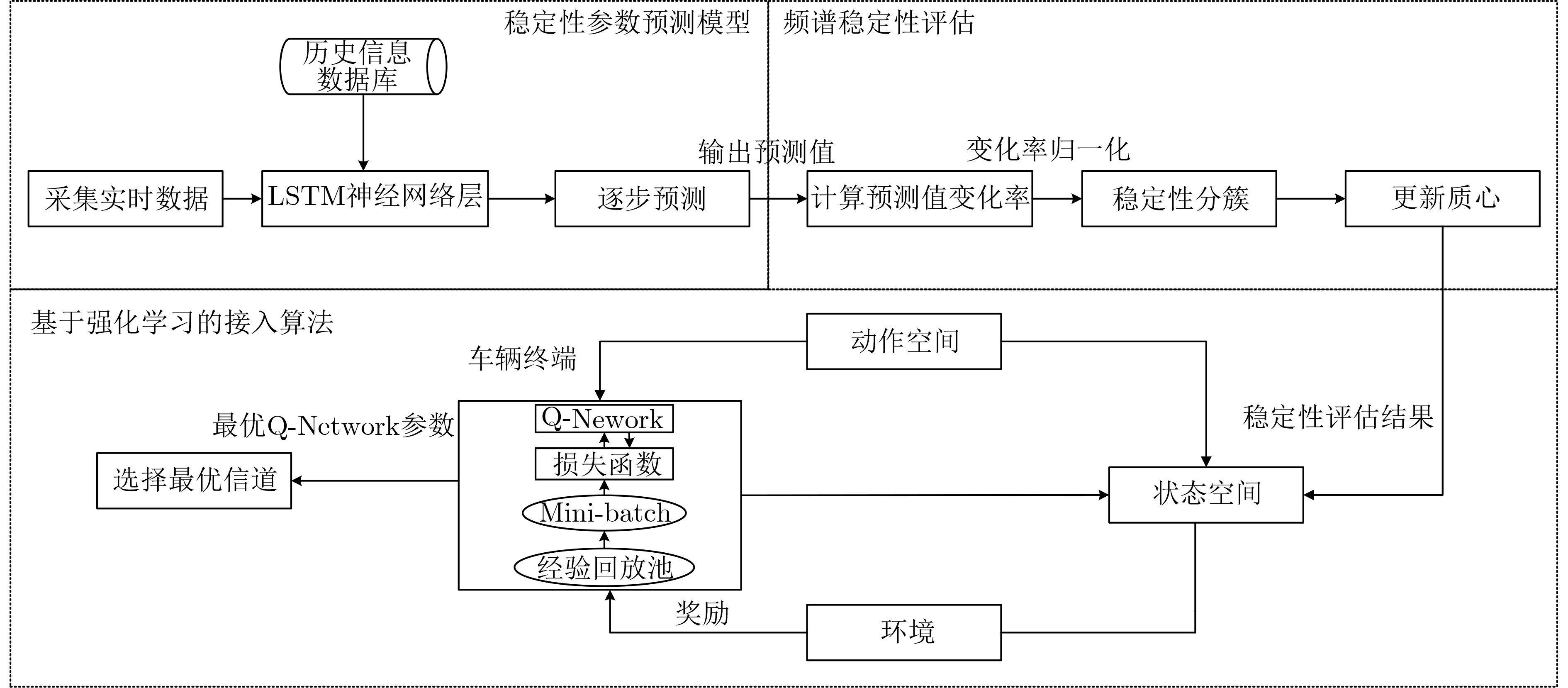
摘要: 在带频谱认知的车联网中，由于车辆终端的高动态移动性和无线电环境的复杂性，使频谱的稳定性难以评估。该文提出一种评估频谱稳定性的动态频谱接入算法。首先，基于信噪比、接收信号强度和带宽参数，利用长短期记忆神经网络预测出参数在未来1个周期内多时刻的值，并计算各参数1个周期的变化率，将结果作为频谱稳定性的评估指标。其次，利用K-Means算法对变化率向量进行聚类，构建稳定性评估模型。再次，根据稳定性评估结果重构了状态空间和奖励函数，提出一种基于强化学习的动态频谱接入算法。最后，实验结果表明，所提算法能够满足不同车辆终端业务的稳定性需求，提高频谱资源的利用率，同时降低频谱接入过程中的碰撞概率。

关键词:

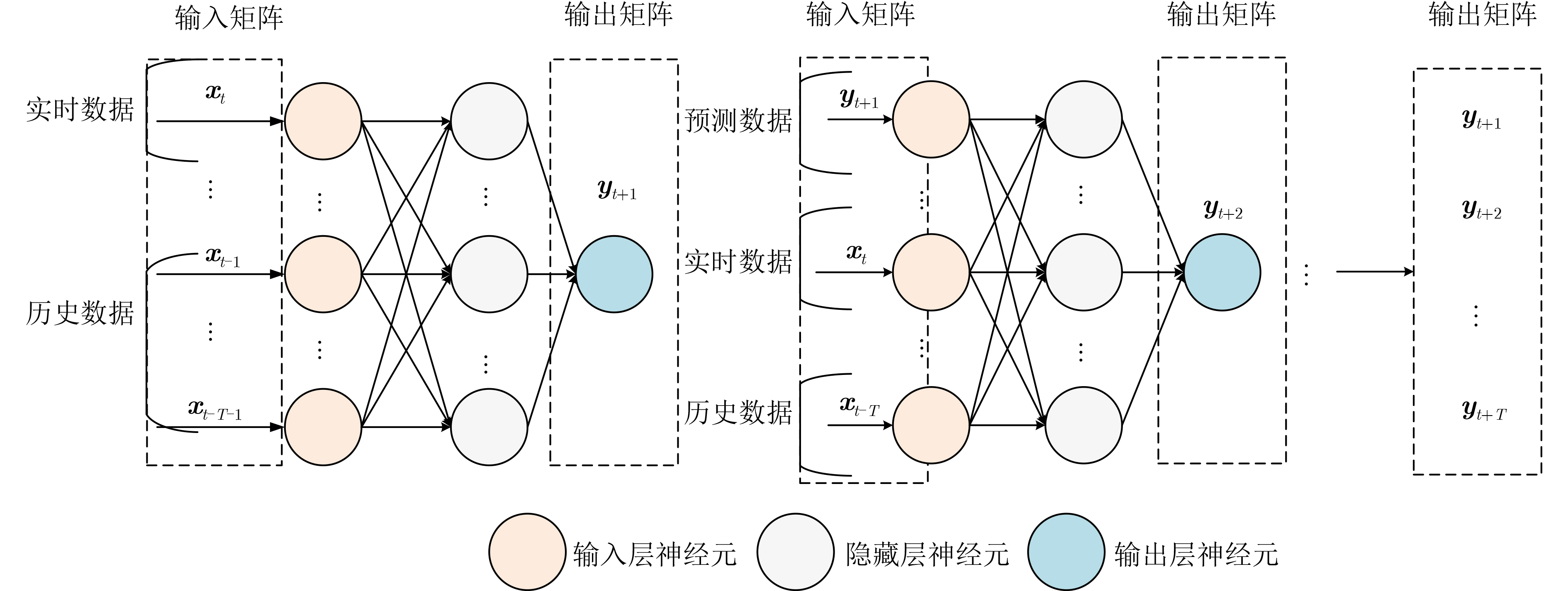
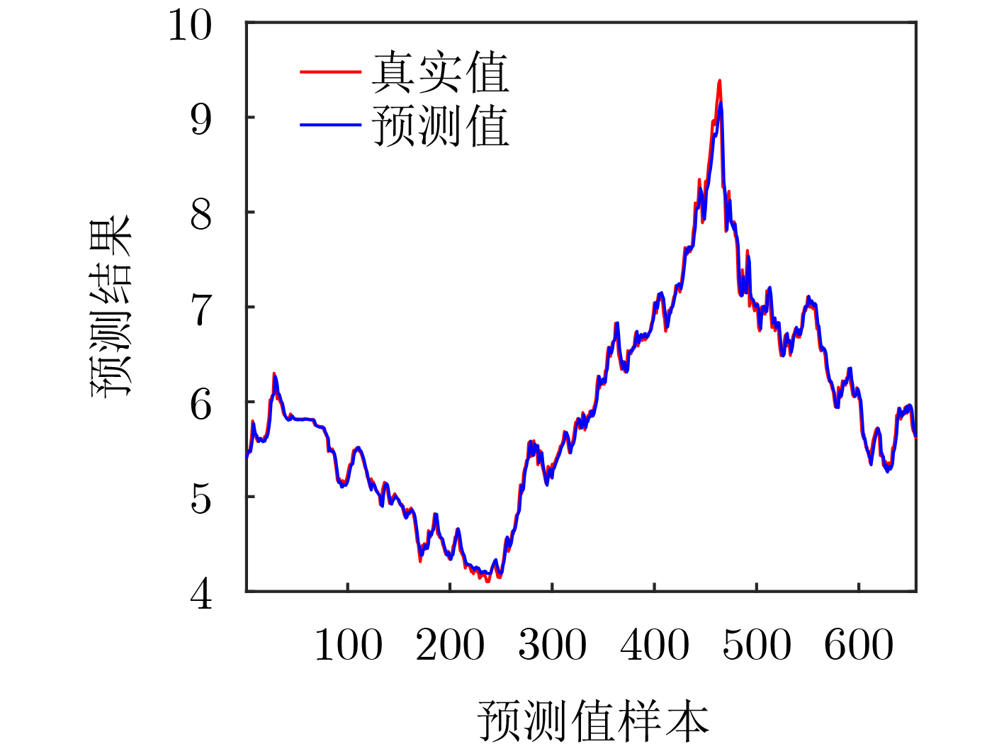
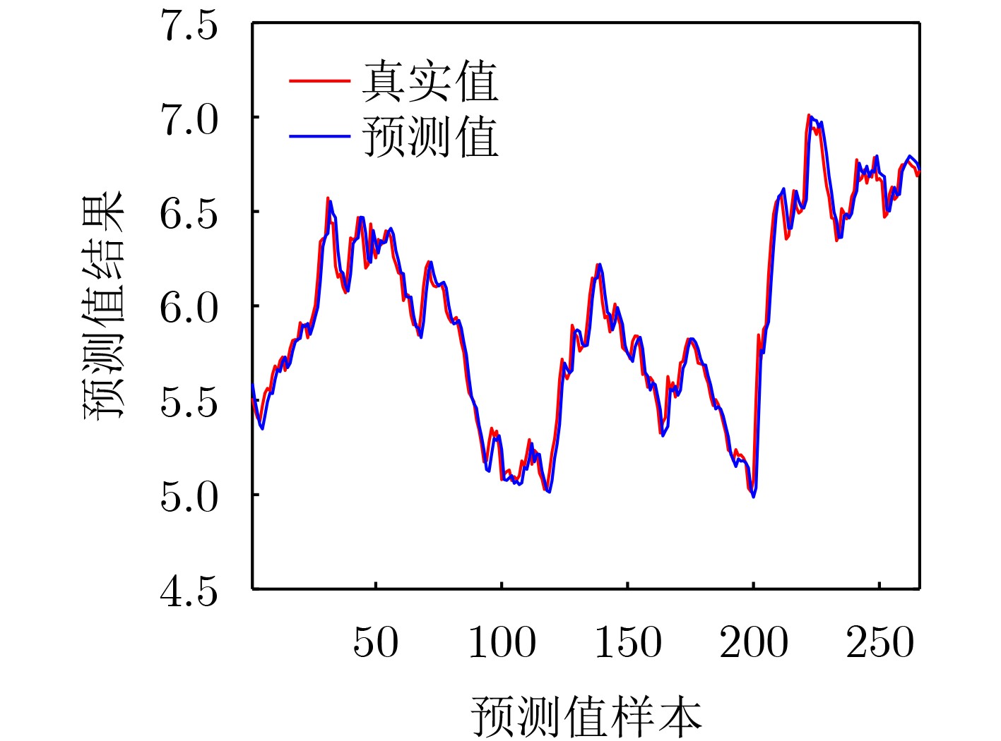
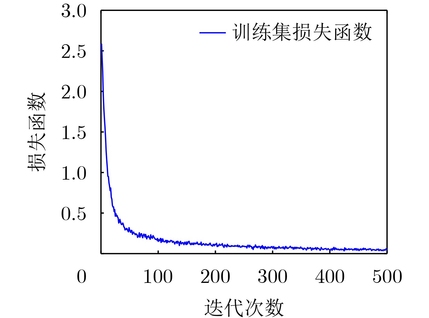
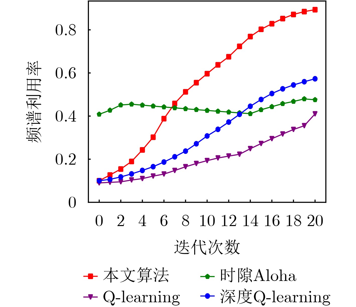
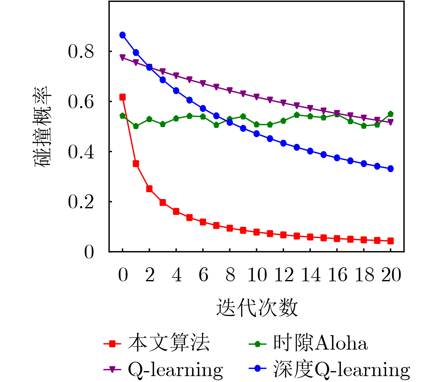
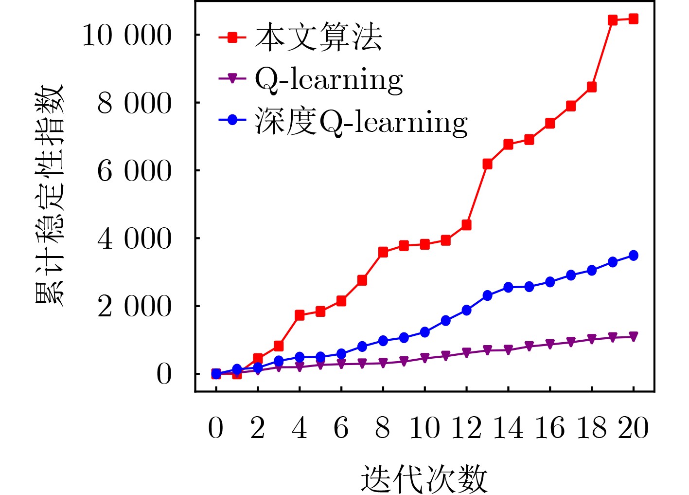
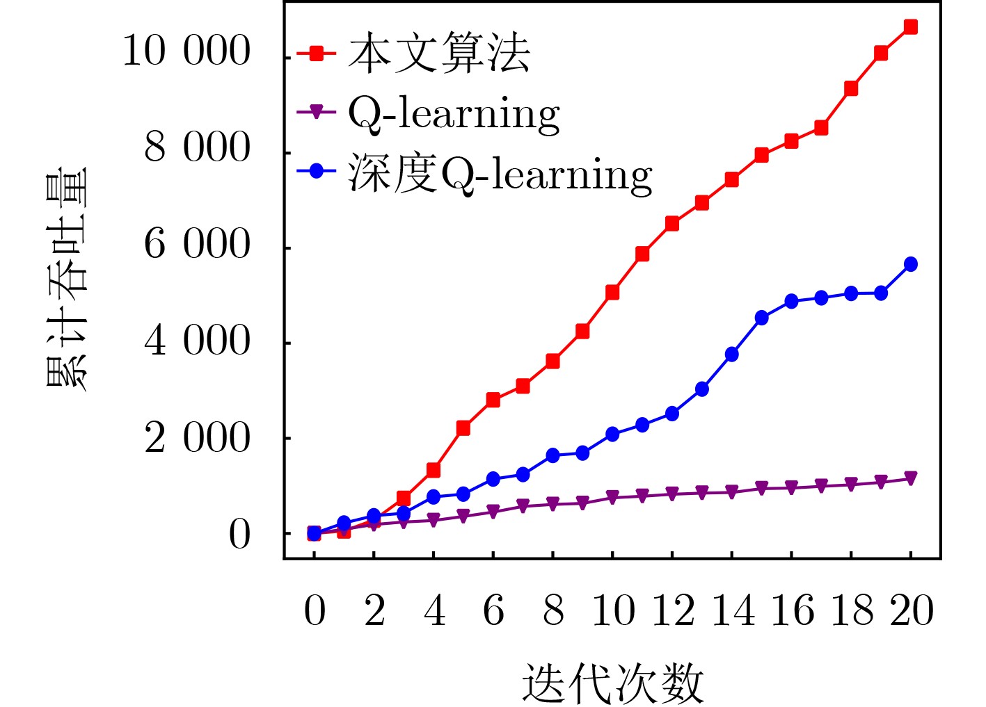
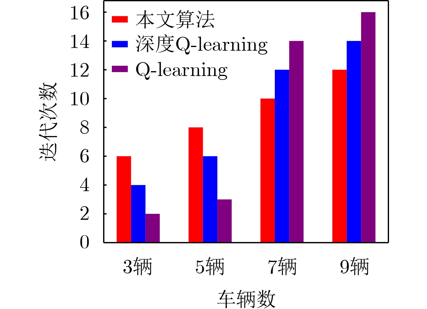
Abstract: Objective With the exponential growth of vehicle terminals and the widespread adoption of cognitive vehicular network applications, the existing licensed spectrum resources are inadequate to meet the communication demands of Cognitive Vehicular Networks (CVN). The rapid development of CVN and the increasing complexity of vehicular communication scenarios have intensified spectrum resource scarcity. Dynamic Spectrum Access (DSA) technology has emerged as a key solution to alleviate this scarcity by enabling efficient use of underutilized spectrum bands. While current DSA algorithms ensure basic spectrum utilization, they struggle to comprehensively evaluate spectrum stability and meet the differentiated stability requirements of vehicular network applications. For example, safety-critical applications such as collision avoidance systems demand ultra-reliable, low-latency communication, while infotainment applications prioritize high throughput. This paper proposes a novel framework integrating spectrum stability assessment with deep reinforcement learning. The framework constructs a multi-dimensional parameter-based model for spectrum stability, designs a reinforcement learning architecture incorporating gated mechanisms and dueling neural networks, and establishes a dynamically adaptive reward function to enable intelligent spectrum resource allocation. This research offers a solution for vehicular network spectrum management that combines theoretical depth with practical engineering value, paving the way for more reliable and efficient vehicular communication systems. Methods This study employs an integrated approach to address the spectrum allocation challenges in CVN. A time-series prediction model is developed using Long Short-Term Memory (LSTM) neural networks, which leverage three-dimensional time-series data of Signal-to-Noise Ratio (SNR), Received Signal Strength (RSS), and bandwidth to make multi-step predictions for future cycles. The rate of change for each parameter is calculated as a stability evaluation metric, providing a quantitative measure of spectrum stability. To ensure consistency in the evaluation process, the rate of change for each parameter is normalized using Min-Max normalization, and the standardized results are input into the K-Means algorithm for stability clustering of the rate-of-change vectors. By calculating the centroid coordinates of each cluster and their norms, a stability index is derived, forming the stability assessment model. Building upon the Deep Q-Network (DQN), a Gated Recurrent Unit (GRU) is introduced to create a temporal state encoder that captures the temporal dependencies in spectrum data. Additionally, a Dueling Network architecture is employed to decouple the state value and action advantage functions, enabling more accurate estimation of the long-term value of spectrum allocation decisions. The reward function incorporates trade-off coefficients to achieve a reasonable allocation of spectrum resources with different stability levels, ensuring a balance between spectrum utilization and collision probability while meeting the diverse stability requirements of vehicular network applications. The proposed framework is designed to be scalable and adaptable to various vehicular network scenarios, including urban, highway, and rural environments. Results and Discussions Simulation results show that the optimized stepwise prediction algorithm significantly improves performance. In both the training and test sets, the algorithm achieves a Mean Squared Error (MSE) of less than 0.1, with no significant overfitting observed (Fig. 5, Fig. 6). This indicates that the algorithm generalizes well to unseen data, making it suitable for real-world deployment. Additionally, the loss function of the proposed algorithm decreases significantly as the number of iterations increases, converging around 150 iterations (Fig. 7). The prediction accuracy also stabilizes around 150 iterations (Fig. 8), suggesting that the algorithm achieves consistent performance within a reasonable training period. These results demonstrate that the proposed prediction algorithm can deliver high-accuracy multi-step predictions for stability parameters across a sufficient number of channels, providing a solid foundation for spectrum stability assessment. Furthermore, the proposed access algorithm consistently outperforms comparative algorithms in terms of spectrum utilization over 20 iterations, while maintaining lower collision probabilities (Fig. 9, Fig. 10). As the number of iterations increases, the cumulative stability index and throughput of the proposed algorithm steadily improve, exceeding the performance of comparative algorithms at all stages. This demonstrates that the proposed algorithm can meet the diverse requirements of vehicle terminals for channel stability and throughput, while ensuring high spectrum utilization and low collision probability. As the number of vehicle terminals increases, the proposed algorithm exhibits faster convergence compared to other algorithms, confirming its robustness in large-scale scenarios. These findings highlight the potential of the proposed framework to meet the growing demands of next-generation vehicular networks. Conclusions This study proposes an integrated "evaluation-decision-optimization" spectrum management paradigm for CVN. By proposing a multi-dimensional time-series feature-based spectrum stability quantification framework and designing a hybrid deep reinforcement learning architecture incorporating gated mechanisms and dueling networks, the research addresses the critical challenge of balancing spectrum efficiency with stability in dynamic vehicular environments. The development of an interpretable reward function enables intelligent spectrum allocation that adapts to diverse quality-of-service requirements, ensuring that both safety-critical and non-safety-critical applications receive the necessary resources. Experimental results show significant improvements in spectrum utilization, collision probability, and system throughput compared to traditional approaches, while maintaining robust performance in large-scale scenarios. These findings advance the theoretical understanding of spectrum management in CVN and provide a practical framework for implementing adaptive DSA solutions in next-generation intelligent transportation systems. Future research will explore extending the proposed framework to support multi-agent scenarios, where multiple vehicles and infrastructure nodes collaboratively optimize spectrum allocation. Additionally, integrating edge computing and federated learning techniques could further enhance the scalability and efficiency of the framework. The proposed methodology offers a scalable and efficient approach to spectrum resource allocation, paving the way for more reliable and high-performance vehicular communication networks.

Key words:

1. 引言

太赫兹(0.1～10 THz)通信拥有超宽带宽，可实现高速率数据传输、高精度目标感知和定位。但是，太赫兹信号传输损耗高，尤其当太赫兹信号被障碍物遮挡时，其通信和感知性能会急剧下降^[1–3]。为此，可以部署由大量低功耗无源元件组成的可重构智能反射面(Reflecting Intelligent Surface, RIS)以智能改变无线传输环境，提供额外的反射路径，解决视距(Line of Sight, LoS)链路阻塞问题，增强接收信号能量，提高太赫兹通感性能^[4]。因此，RIS辅助太赫兹感知具有广阔的应用前景^[5–7]。一般来说，RIS元件的结构比较简单，通常配备与频率无关的移相电路，只能调整反射信号的振幅和相位。因此，在RIS辅助太赫兹系统中，RIS每个反射元件仅能控制单一载波的波束方向，而对于多载波RIS系统将出现不同子载波波束指向不同方向，此现象称为波束色散效应。尽管波束色散在通信中会降低用户接收的波束增益^[8–10]，但是却可以利用色散特性提升感知能力。例如，文献[11]提出一种名为太赫兹棱镜(THz prism)的新型相控阵天线结构，利用波束色散效应，实现基于频率的波束扩展。文献[12]利用实时延(True Time Delay, TTD)自由控制近场中波束色散范围和轨迹，通过频域波束色散效应进行目标定位。文献[13]在基站(Base Station, BS)波束色散基础上，引入波束分裂效应来扩大波束覆盖范围，从而增加单次感知范围。

基于上述分析，本文提出了联合太赫兹RIS处的波束色散和分裂快速感知方法，具体而言，基于RIS辅助太赫兹感知系统利用太赫兹RIS处产生的波束色散效应，通过调整波束范围进行区域感知。然后，设置大间距RIS反射元件产生波束分裂效应以扩大感知范围，并联合波束色散和分裂进行多个子区域感知。通过优化RIS处的TTD和反射单元相移，实现RIS处的波束色散覆盖单一子区域，波束分裂无缝覆盖多个子区域。最后，根据RIS处配备的有源感知元件接收到回波信号推导出目标所在方向估计值及其均方根误差(Root Mean Square Error, RMSE)，仿真结果表明了所提快速感知方案的有效性。

2. 系统模型

考虑如所示的RIS辅助太赫兹感知系统模型，其中单天线感知BS与感知区域间的直接链路被障碍物等阻断，需借助RIS辅助感知。其中RIS是由无源和有源元件共同组成，无源元件主要是对信号进行反射，简称“-RE”元件；有源元件主要是接收并分析回波信号，简称“-SE”元件。具体感知过程如下：由 $R$ 个RE元件组成的均匀线性反射阵列(Uniform Linear Array, ULA)将感知BS发射的感知信号反射至感知区域，由 ${R_{\mathrm{s}}}$ 个SE元件组成的ULA接收回波并进行目标方向估计。

图 1 RIS辅助太赫兹感知系统模型

下载: 全尺寸图片幻灯片

$g(t)$ 和 $f(t)$ 分别表示BS-RIS链路和RIS-目标链路的时域信道向量。基于远场假设， BS到第 $r$ 个RIS元件的第 ${l_1}$ 路径时延、第 $r$ 个元件到目标的第 ${l_2}$ 路径时延 ${\tau _{{l_{{\text{1,}}r}}}}$ , ${\tau _{{l_{{\text{2}},r}}}}$ 分别表示为

${\tau _{{l_{1,r}}}} = {\tau _{{l_{1,1}}}} + (r - 1)\frac{{d\sin \theta _{{\text{BR}}}^{{l_1}}}}{{\text{c}}} = {\tau _{{l_{1,1}}}} + (r - 1)\frac{{\phi _{{\text{BR}}}^{{l_1}}}}{{{f_{\text{c}}}}}$

(1)

${\tau _{{l_{2,r}}}} = {\tau _{{l_{2,1}}}} + (r - 1)\frac{{d\sin \theta _{{\text{RT}}}^{{l_2}}}}{{\text{c}}} = {\tau _{{l_{2,1}}}} + (r - 1)\frac{{\phi _{{\text{RT}}}^{{l_2}}}}{{{f_{\text{c}}}}}$

(2)

其中， $\phi _{{\text{BR}}}^{{l_1}} = d\sin \theta _{{\text{BR}}}^{{l_1}}/{\lambda _{\text{c}}}$ , $\phi _{{\text{RT}}}^{{l_2}} = d\sin \theta _{{\text{RT}}}^{{l_2}}/{\lambda _{\text{c}}}$ 分别表示BS的归一化离开角(Angle of Departure, AoD)、到达角(Angle of Arrival, AoA)。假设 $d$ , ${\text{c}}$ , ${\lambda _{\text{c}}}$ , ${f_{\text{s}}}$ , ${f_{\text{c}}}$ 分别表示相邻RIS元件间距、光速、波长、带宽和载波中心频率。因此， BS到第 $r$ 个RIS元件信道脉冲响应、第 $r$ 个RIS元件到目标的信道脉冲响应可表示为 ${g_r}(t) = {\alpha _{{l_1}}}{{\text{e}}^{{{ - {\mathrm{j}}}}2{\pi }{f_{\text{c}}}{\tau _{{l_{1,r}}}}}}\delta (t - {\tau _{{l_{1,r}}}})$ , ${f_r}(t) = {\alpha _{{l_2}}}{{\text{e}}^{{{ - {\mathrm{j}}}}2{\pi }{f_{\text{c}}}{\tau _{{l_{2,}}_r}}}}\delta (t - {\tau _{{l_{2,r}}}})$ 。则目标在第 $r$ 个RIS元件处接收的信号可表示为

$\begin{split} {y_r}{\text{(}}t) =\;& {f_r}(t)*({\theta _r}{g_r}(t)*s(t)) + n\\ =\;& {\theta _r}\sum\limits_{{l_1} = 1}^{{L_1}} {\sum\limits_{{l_2} = 1}^{{L_2}} {{\alpha _{{l_1}}}{\alpha _{{l_2}}}{{\text{e}}^{{{ - {\mathrm{j}}}}2{\pi }{f_{\text{c}}}{\tau _{{l_{1,r}}}}}}} } \\ & \cdot{{\text{e}}^{{-\text{j}}2{\pi }{f_{\text{c}}}{\tau _{{l_{2,r}}}}}}{\text{s}}(t - {\tau _{{l_{1,r}}}} - {\tau _{{l_{2,r}}}}) + n\\ =\;& {\theta _r}{h_r}(t)*s(t) + n \end{split}$

(3)

其中， $s(t)$ 为BS发出的信号， $n$ 为加性复高斯噪声。记 ${\boldsymbol{\theta}} = {[{\theta _{\text{1}}},{\theta _{\text{2}}}, \cdots ,{\theta _R}]^{\text{T}}} \in {\mathbb{C}^{R \times 1}}$ , ${\theta _r} = {\beta _r}{{\text{e}}^{{\text{j}}{\phi _r}}}$ 分别表示RIS反射系数向量和第 $r$ 个RIS元件的反射系数。 ${\beta _r} \in [0,1]$ 和 ${\phi _r} \in [0,2{\pi })$ 分别表示第 $r$ 个反射单元的幅度和相移。为最大化RIS的信号功率和简化硬件设计，通常固定 ${\beta _r} = 1,{\forall _r}$ 。因此， ${\boldsymbol{\theta}}$ 满足 ${\boldsymbol{\theta}} = [{{\text{e}}^{{\text{j}}{\phi _{\text{1}}}}}, {{\text{e}}^{{\text{j}}{\phi _2}}}, \cdots ,{{\text{e}}^{{\text{j}}{\phi _R}}}]^{\text{T}}$ 。 $*$ 表示卷积运算，级联BS-RIS-目标在第 $r$ 元件的第 $l$ 条路径处的时域信道脉冲响应 ${h_r}(t)$ 表示为

$\begin{split} {h_r}(t) =\;& \sum\limits_{{l_1} = 1}^{{L_1}} \sum\limits_{{l_2} = 1}^{{L_2}} {\alpha _{{l_1}}}{\alpha _{{l_2}}}{{\text{e}}^{{{ - {\mathrm{j}}2\pi }}{f_{\text{c}}}{\tau _{{l_{1,r}}}}}}{{\text{e}}^{{{ - {\mathrm{j}}2\pi }}{f_{\text{c}}}{\tau _{{l_{2,r}}}}}}\\ &\cdot \delta (t - {\tau _{{l_{1,r}}}} - {\tau _{{l_{2,r}}}}) \end{split}$

(4)

对式(4)进行傅里叶变换，频域信道响应 ${h_r}(f)$ 可以表示为

$\begin{split} {h_{\text{r}}}(f) \;& = \int\limits_{ - \infty }^{ + \infty } {{h_r}(t){{\text{e}}^{{{ - {\mathrm{j}}}}2{\pi }ft}}{\mathrm{d}}t} \\ & = \sum\limits_{{l_1} = 1}^{{L_1}} {\sum\limits_{{l_2} = 1}^{{L_2}} {\alpha {{\text{e}}^{{{ - {\mathrm{j}}2\pi }}(r - 1){\phi _{{l_3}}}(1 + \frac{f}{{{f_{\text{c}}}}})}}{{\text{e}}^{{{ - {\mathrm{j}}2\pi }}f{\tau _{{l_3}}}}}} } \end{split}$

(5)

其中， $\alpha = {\alpha _{{l_1}}}{\alpha _{{l_2}}}$ , ${\phi _{{l_{\text{3}}}}} = \phi _{{\text{BR}}}^{{l_1}} - \phi _{{\text{RT}}}^{{l_2}}$ , ${\tau _{{l_3}}} = {\tau _{{l_{1,r}}}} + {\tau _{{l_{2,r}}}}$ 分别定义为级联BS-RIS-目标信道等效复路径增益、角度和时延。假设 ${L_1} = 1$ , ${L_2} = 1$ 。则级联信道可重新表示为

${h_r}(f) = \alpha {{\text{e}}^{{{ - {\mathrm{j}}}}2{\pi }(r - 1)\phi (1 + \frac{f}{{{f_{\text{c}}}}})}}{{\text{e}}^{{{ - {\mathrm{j}}}}2{\pi }f{\tau _{_0}}}}$

(6)

其中， $\phi = d(\sin {\theta _{{\text{BR}}}} - \sin {\theta _{{\text{RT}}}})/{\lambda _{\text{c}}}$ , ${\tau _0} = {\tau _0}^{{\text{BR}}} + {\tau _0}^{{\text{RT}}}$ 分别为单路径级联BS-RIS-目标信道的等效角度、等效时延，记 $v = \sin {\theta _{{\text{BR}}}} - \sin {\theta _{{\text{RT}}}}$ 。级联信道矢量 ${\boldsymbol{h}}(f) = {[{h_{\text{1}}}(f),{h_{\text{2}}}(f),\cdots,{h_R}(f)]^{\text{T}}}$ 具体可以描述为

${\boldsymbol{h}}(f) = \alpha {\boldsymbol{a}}(f,v){{\text{e}}^{ - {\text{j}}2{\pi }f{\tau _0}}}$

(7)

其中空间转向矢量可表示为 ${\boldsymbol{a}}(f,v) = [1,{{\text{e}}^{{{ - {\mathrm{j}}}}2{\pi }\frac{d}{{{\lambda _{\text{c}}}}}(1 + \frac{f}{{{f_{\text{c}}}}})v}}, \cdots, {{\text{e}}^{{{ - {\mathrm{j}}}}2{\pi }\frac{d}{{{\lambda _{\text{c}}}}}(R - 1)(1 + \frac{f}{{{f_{\text{c}}}}})v}}]^{\text{T}}$ 。

2.1 波束色散效应

在传统阵列信号处理中，为避免相位模糊，通常情况下假设相邻元件间距 $d = {\lambda _{\text{c}}}/2$ ，则级联BS-RIS-目标频域信道响应 ${\boldsymbol{h}}(f)$ 可以表示为

${{\boldsymbol{h}}_1}(f) = \alpha {{\boldsymbol{a}}_1}(f,v){{\text{e}}^{{{ - {\mathrm{j}}}}2{\pi }f{\tau _0}}}$

(8)

其中，空间转向矢量 ${{\boldsymbol{a}}_1}(f,v) = [1,{{\text{e}}^{{{ - {\rm j}\pi }}v(1 + \frac{f}{{{f_{\text{c}}}}})}},\cdots, {{\text{e}}^{{{ - {\rm j}\pi }}v(R - 1)(1 + \frac{f}{{{f_{\text{c}}}}})}}]^{\text{T}}$ 。频率 $f$ 处阵列增益可表示为

$\begin{split} {g_{\text{1}}}(f,v,{\varphi _r}) \;&= \left| {{\boldsymbol{a}}_1^{\text{T}}(f,v){\boldsymbol{\theta}} } \right| \\ & = \left| {\sum\limits_{r = 1}^R {{{\text{e}}^{{{ - {\rm j}\pi }}(r - 1)v(1 + \frac{f}{{{f_{\text{c}}}}})}}{{\text{e}}^{{\text{j}}{\phi _r}}}} } \right| \\ & = \left| {\sum\limits_{r = 1}^R {{{\text{e}}^{{\text{j}}[{\phi _r} - {\pi }(r - 1)(1 + \frac{f}{{{f_{\text{c}}}}})v]}}} } \right| \end{split}$

(9)

假设 $v = {v_{\text{c}}}$ ， ${v_{\text{c}}}$ 为中心频率处的等效方向，此时 $f = {f_{\text{c}}}$ 。为最大化归一化阵列增益 ${g_1}({f_{\text{c}}},{v_{\text{c}}},{\phi _r})$ ，可得 ${\phi _{r{\text{,c}}}} = 2{\pi }(r - 1){v_{\text{c}}}$ 。因此，反射系数矢量可以表示为 ${{\boldsymbol{\theta}} _{\text{c}}} = {[1,{{\text{e}}^{{\text{j}}2{\pi }{v_{\text{c}}}}},\cdots,{{\text{e}}^{{\text{j}}2{\pi }(R - 1){v_{\text{c}}}}}]^{\text{T}}}$ 。在频率 $f$ 下任意方向 $v$ 下获得的波束阵列增益可表示为

$\begin{split} {g_{_1}}(f,v,{\varphi _{r{\text{,c}}}}) =\;& \left| {{\boldsymbol{a}}_1^{\text{T}}(f,v){{\boldsymbol{\theta}} _{\text{c}}}} \right| \\ =\;& \left| {\sum\limits_{r = 1}^R {{{\text{e}}^{{\text{{{j}}\pi }}(r - 1)[2{v_{\text{c}}} - (1 + \frac{f}{{{f_{\text{c}}}}})v]}}} } \right| \\ =\;& \left| {\frac{{\sin \left(\dfrac{{R{\pi }}}{2}\rho \right)}}{{\sin \left(\dfrac{{\pi }}{2}\rho \right)}}{{\text{e}}^{{\text{j}}\frac{{(R - 1){\pi }}}{2}\rho }}} \right| \end{split}$

(10)

其中， $\rho = 2{v_{\text{c}}} - \left(1 + {f}/{{{f_{\text{c}}}}}\right)v$ ，利用等式 $\displaystyle\sum\nolimits_{r = 1}^R {{{\text{e}}^{{\text{j}}(r - 1){\pi }x}}} = \left({{\sin \left(\dfrac{{R{\pi }}}{2}x\right)}}/{{\sin \left(\dfrac{{\pi }}{2}x\right)}}\right){{\text{e}}^{{\text{j}}\frac{{(R - 1){\pi }}}{2}x}}$ 。为满足波束增益最大化使 $\rho = 0$ ，此时，波束方向与频率之间的关系为 $v = \dfrac{2}{{1 + f/{f_{\text{c}}}}}{v_{\text{c}}}$ 。由于在窄带情况下 $f/{f_{\text{c}}} \approx 1$ ，则在所有频率下波束的方向 $v \approx {v_{\text{c}}}$ ，这意味着所有子载波上的波束将聚焦在同一方向上，并且每个子载波的最大波束增益可以在该方向上获得。然而，对于太赫兹系统， $f/{f_{\text{c}}} \approx 1$ 不再成立，出现明显的波束色散效应，其波束图样如图2所示。

图 2 波束色散效应下的波束图样

下载: 全尺寸图片幻灯片

2.2 波束分裂效应

当元件间距大于 ${\lambda _{\text{c}}}/2$ ，由于空间导向矢量的范德蒙德结构而发生相位模糊，根据具体数值的不同，将会产生不同数量的和主瓣强度相当的旁瓣，称为“栅瓣”，波束分裂效应的波束图样如所示。具体地，假设间距为 $d = P{\lambda _{\text{c}}}/2$ ，其中 $P$ 为分裂系数，取值为正整数。改变RIS元件间距 $d$ 的有效方法是部署具有半波长间距的RIS阵列，通过控制RIS元件结构中的二极管的通断来调整元件之间的间距，内部电路图如所示^[14]，根据 $d$ 的不同实现不同间距的子阵列，如图5所示。

图 3 波束分裂效应下的波束图样(

$P = 3$ )

下载: 全尺寸图片幻灯片

图 4 RIS元件中有关二极管结构电路图

下载: 全尺寸图片幻灯片

图 5 RIS元件不同间距的阵列图

下载: 全尺寸图片幻灯片

将 $d = P{\lambda _{\text{c}}}/2$ 代入式(7)得，级联BS-RIS-目标频域信道响应 ${\boldsymbol{h}}(f)$ 可以表示为

${{\boldsymbol{h}}_2}(f) = \alpha {{\boldsymbol{a}}_2}(f,v){{\text{e}}^{{{ - {\mathrm{j}}}}2{\pi }f{\tau _0}}}$

(11)

其中，空间转向矢量 ${{\boldsymbol{a}}_2}(f,v) = [1,{{\text{e}}^{{{ - {\rm j}\pi }}Pv(1 + \frac{f}{{{f_{\text{c}}}}})}},\cdots, {{\text{e}}^{{{ - {\rm j}\pi }}Pv(R - 1)(1 + \frac{f}{{{f_{\text{c}}}}})}}]^{\text{T}}$ 。与2.1节分析类似，假设 $f = {f_{\text{c}}}$ 时， $v = P{v_{\text{c}}}$ ，此时设置 ${\phi _{r{\text{,c}}}} = 2{\pi }(r - 1) P{v_{\text{c}}}$ 。反射系数矢量 ${{\boldsymbol{\theta}} _{\text{c}}}$ 可以表示为 ${{\boldsymbol{\theta}} _{\text{c}}} = [1,{{\text{e}}^{{{{\mathrm{j}}2\pi }}P{v_{\text{c}}}}},\cdots, {{\text{e}}^{{\text{j}}2{\pi }(R - 1)P{v_{\text{c}}}}}]^{\text{T}}$ 。在频率 $f$ 下任意方向 $v$ 下获得的波束阵列增益可表示为

$\begin{split} {g_2}(f,v,{\phi _{r{\text{,c}}}})\;& = \left| {{{\boldsymbol{a}}_2}^{\text{T}}(f,v){{\boldsymbol{\theta}} _{\text{c}}}} \right| \\ & = \left| {\sum\limits_{r = 1}^R {{{\text{e}}^{{{{\mathrm{j}}\pi }}(r - 1)P[2{v_{\text{c}}} - (1 + \frac{f}{{{f_{\text{c}}}}})v]}}} } \right|\\ &= \left| {\frac{{\sin \left(\dfrac{{R{\pi }}}{2}\rho \right)}}{{\sin \left(\dfrac{{\pi }}{2}\rho \right)}}{{\text{e}}^{{\text{j}}\frac{{(R - 1){\pi }}}{2}\rho }}} \right| \end{split}$

(12)

其中， $\rho = P\left(2{v_{\text{c}}} - \left(1 + {f}/{{{f_{\text{c}}}}}\right)v\right)$ 。可以看出，为满足波束增益最大化应当使 $\rho = 0$ ，此时波束方向与频率之间的关系为 $v' = \dfrac{2}{{1 + f/{f_{\text{c}}}}}{v_{\text{c}}}$ 。

虽然波束分裂波束方向与频率关系式与上文波束色散分析形式相同，但原理上并不相同。主要区别在于波束色散效应使波束方向随频率的变化而变化，但是每个载波上只有一个波束方向。然而，波束分裂效应因为栅瓣的存在，使同一频率处的波束分散为多个方向，可以看成一个波束分裂为多个指向不同的波束，其分裂个数与系数 $P$ 有关。相邻RIS元件间产生的相位差为 $\Delta \phi = 2{\pi }\dfrac{{d{\text{sin}}{\theta _{{\text{BR}}}}}}{{{\lambda _{\text{c}}}}}$ 。栅瓣波束方向记为 $v = \arcsin \left(\dfrac{{\Delta \phi }}{{2{\pi }}}\dfrac{{{\lambda _c}}}{d}\right)$ ，由周期性得 $v = \arcsin \left(\dfrac{{\Delta \varphi + 2{\pi }m}}{{2{\pi }}}\dfrac{{{\lambda _{\text{c}}}}}{d}\right)$ , $m \in \forall \mathbb{Z}$ 。因此，与 $P$ 有关的波束方向表达式为 $v = \arcsin \left( \dfrac{{2{\pi }\dfrac{{d{\text{sin}}{\theta _{{\text{BR}}}}}}{{{\lambda _{\text{c}}}}} + 2{\pi }m}}{{2{\pi }}}\dfrac{{{\lambda _{\text{c}}}}}{d} \right) = \arcsin \left(\sin {\theta _{{\text{BR}}}} + \dfrac{{2m}}{P}\right)$ 。由于其中 $\arcsin x$ 函数的特殊性质，定义域 $x \in [ - 1,1]$ ，因此限制了 $m$ 的取值。当 $m = 0$ 时，无论 $P$ 取何值，该式均成立，即 $m = 0$ 是通解。当 $P = 1$ 时，即 $d = {\lambda _{\text{c}}}/2$ ，得 $v = \arcsin (\sin {\theta _{{\text{BR}}}} + 2m)$ ，由于 $\sin{\theta _{{\text{BR}}}} \in [ - 1,1]$ ，所以 $m$ 有且只有 $m = 0$ 这1个解，此时 $v = {\theta _{{\text{BR}}}}$ ,此时仅存在波束色散效应。当 $P = 2$ 时，即 $d = 2{\lambda _{\text{c}}}/2$ ，得 $v = \arcsin (\sin {\theta _{{\text{BR}}}} + m)$ ，根据选取 ${\theta _{{\text{BR}}}}$ 不同， $m$ 可取的值也有所不同。当 $\sin{\theta _{{\text{BR}}}} \in (0,1]$ ，存在 $m = 0$ 和 $m = - 1$ 两个解， ${v_1} = \arcsin (\sin {\theta _{{\text{BR}}}})$ , ${v_2} = \arcsin (\sin {\theta _{{\text{BR}}}} - 1)$ ，则 $P = 2$ 时波束会分裂成两个角度。当 $\sin {\theta _{{\text{BR}}}} = 0$ 时，解为 $m = 0$ , $m = - 1$ 和 $m = 1$ ，此时波束会分裂成3个角度。因此，波束分裂不仅与分裂系数 $P$ 有关，还与角度选取有关。

3. 基于TTD的RIS波束色散和分裂

本节分析不同RIS单元间距下基于TTD波束色散和分裂影响。如图6所示，每个RIS单元上连接一个TTD，TTD是频率相关的宽带器件，可通过改变信号的传播时延，来调整波束色散和分裂程度。

图 6 基于TTD的RIS元件结构图

下载: 全尺寸图片幻灯片

第 $r$ 个RIS单元和TTD连接组合的时域响应为 ${{\text{e}}^{{\text{j}}{\phi _r}}}\delta (t - {t_r})$ ， ${t_r}$ 为第 $r$ TTD引入的延时，则对应的频域响应表示为 ${b_r} = {{\text{e}}^{{\text{j}}{\phi _r}}}{{\text{e}}^{{-\text{j}}2{\pi }f{t_r}}}$ ，相应频域响应矢量为 ${\boldsymbol{b}} = [{{\text{e}}^{{\text{j}}{\phi _1}}}{{\text{e}}^{{{ - {\mathrm{j}}}}2{\pi }f{t_1}}},\cdots,{{\text{e}}^{{\text{j}}{\phi _r}}}{{\text{e}}^{{{ - {\mathrm{j}}}}2{\pi }f{t_r}}},\cdots, {{\text{e}}^{{\text{j}}{\phi _R}}}{{\text{e}}^{{{ - {\mathrm{j}}}}2{\pi }f{t_R}}}]^{\text{T}}$ 。由上文分析BS-RIS-目标级联信道响应式级联信道响应重新表述为

${\boldsymbol{h}}'(f) = \alpha {\boldsymbol{a}}(\varTheta (f)){{\text{e}}^{{{ - {\mathrm{j}}}}2{\pi }f{\tau _0}}}$

(13)

其中， ${\boldsymbol{a}}(\varTheta (f)) = [1,{{\text{e}}^{{{ - {\mathrm{j}}2\pi }}\frac{d}{{{\lambda _{\text{c}}}}}v(2 + \frac{f}{{{f_{\text{c}}}}})}},\cdots$ , ${{\text{e}}^{{{ - {\mathrm{j}}2\pi }}(R - 1)\frac{d}{{{\lambda _{\text{c}}}}}v(2 + \frac{f}{{{f_{\text{c}}}}})}}]^{\text{T}}$ 。定义 $\varTheta (f) = \phi (2 + \frac{f}{{{f_{\text{c}}}}})$ , $f \in [0,{f_{\text{s}}}{\text{]}}$ 。对于有 $M$ 个子载波的正交频分复用 (Orthogonal Frequency Division Multiplexing, OFDM)系统子载波间距为 ${f_{\text{s}}}/M$ ，则第 $m$ 个子载波处的频率可以表示为 ${f_m} = m{f_{\text{s}}}/M$ 。由频率响应矢量 ${\boldsymbol{b}}$ 和空间转向向量 ${\boldsymbol{a}}(\varTheta (f))$ 表示的阵列增益为

$\begin{split} g(f)\;& = \left| {{{\boldsymbol{a}}^{\text{T}}}(\varTheta (f)){\boldsymbol{b}}} \right| \\ & = \left| {\sum\limits_{r = 1}^R {{{\text{e}}^{{{ - {\mathrm{j}}2\pi }}\frac{d}{{{\lambda _{\text{c}}}}}(r - 1)(2 + \frac{f}{{{f_{\text{c}}}}})v}}} {{\text{e}}^{{\text{j}}{\phi _r}}}{{\text{e}}^{{{ - {\mathrm{j}}}}2{\pi }f{t_r}}}} \right| \end{split}$

(14)

3.1 基于TTD的RIS波束色散

首先仅考虑波束色散效应，通过设计TTD和RIS反射系数，可以调整波束色散程度。假设频率 $f$ 从 $0$ 变化到 ${f_{\text{s}}}$ 时，相应波束角度从初始角度 ${v_0}$ 变化到终止角度 ${v_M}$ ， $d = {\lambda _{\text{c}}}/2$ 时的波束阵列增益可表示为

$\begin{split} {g_1}(f) \;&= \left| {{{\boldsymbol{a}}^{\text{T}}}(\varTheta (f)){\boldsymbol{b}}} \right|\\ & = \left| {\sum\limits_{r = 1}^R {{{\text{e}}^{{{ - {\mathrm{j}}\pi }}(r - 1)(2 + \frac{f}{{{f_{\text{c}}}}})v}}} {{\text{e}}^{{\text{j}}{\phi _r}}}{{\text{e}}^{{{ - {\mathrm{j}}2\pi }}f{t_r}}}} \right| \end{split}$

(15)

定义 ${\text{s}}{{\text{v}}_0} = \sin ({\theta _{{\text{BR}}}}) - \sin ({\theta _{{v_{\text{0}}}}})$ 为等效初始角， ${\text{s}}{{\text{v}}_M} = \sin ({\theta _{{\text{BR}}}}) - \sin ({\theta _{{v_{_M}}}})$ 为等效终止角。当 $f = 0$ 时， $v = {\text{s}}{{\text{v}}_0}$ ，最大化 ${g_{\text{1}}}(0) = \left| {\displaystyle\sum\nolimits_{r = 1}^R {{{\text{e}}^{{{ - {\rm j}\pi }}(r - 1)2{\text{s}}{{\text{v}}_0}}}} {{\text{e}}^{{\text{j}}{\phi _r}}}} \right|$ ，可得 ${\phi _1}_r = {\pi }(r - 1)2{\text{s}}{{\text{v}}_0}$ 。当 $f = {f_{\text{s}}}$ 时， $v = {\text{s}}{{\text{v}}_M}$ ，波束增益表示为 ${g_{\text{1}}}({f_{\text{s}}}) = \left| {\displaystyle\sum\nolimits_{r = 1}^R {{{\text{e}}^{{{ - {\rm j}\pi }}(r - 1)(2 + \frac{{{f_{\text{s}}}}}{{{f_{\text{c}}}}}){\text{s}}{{\text{v}}_M}}}} {{\text{e}}^{{{{\mathrm{j}}\pi }}(r - 1)2{\text{s}}{{\text{v}}_0}}}{{\text{e}}^{{{ -{\mathrm{ j}}2\pi }}{f_{\text{s}}}{t_r}}}} \right|$ 。最大化增益可得 ${t_1}_r = \dfrac{{(r - 1)[2{\text{s}}{{\text{v}}_0} - (2 + \dfrac{{{f_{\text{s}}}}}{{{f_{\mathrm{c}}}}}){\text{s}}{{\text{v}}_{_M}}]}}{{2{f_{\text{s}}}}}$ ，则 ${\text{s}}{{\text{v}}_{\text{1}}}_f = \left(\frac{{2{\text{s}}{{\text{v}}_0} - f\dfrac{{[2{\text{s}}{{\text{v}}_0} - (2 + \dfrac{{{f_{\text{s}}}}}{{{f_{\text{c}}}}}){\text{s}}{{\text{v}}_M}]}}{{{f_{\text{s}}}}}}}{{2 + \dfrac{f}{{{f_{\text{c}}}}}}}\right)$ 。因此，任意频率 $f$ 处波束角度 ${\theta _f}$ 可表示为 ${\theta _f} = \arcsin (\sin ({\theta _{{\text{BR}}}}) - {\text{s}}{{\text{v}}_1}_f)$ 。基于TTD波束色散的波束图样如图7所示。

图 7 基于TTD的波束色散

下载: 全尺寸图片幻灯片

3.2 基于TTD的联合波束色散和分裂

由2.1分析可知，波束色散程度与TTD取值有关。当TTD取值固定，波束范围是不可调的。为了解决上述问题，考虑联合利用波束色散和分裂，在载波数目一定情况下，将感知区域分为多个子区域，每个子区域通过波束色散覆盖，不同子区域可以利用波束分裂覆盖。而为了利用波束分裂效应，假设RIS元件 $d = P{\lambda _{\text{c}}}/2$ ，可以通过选择所示的子阵列来实现。同样，假设频率 $f$ 从 $0$ 变化到 ${f_{\text{s}}}$ 时，相应波束角度从初始角度 ${v_0}$ 变化到终止角度 ${v_M}$ 。 $d = P{\lambda _{\mathrm{c}}}/2$ 时的阵列增益为

$\begin{split} {g_2}(f) \;&= \left| {{{\boldsymbol{a}}^{\text{T}}}(\varTheta (f)){\boldsymbol{b}}} \right| \\ & = \left| {\sum\limits_{r = 1}^R {{{\text{e}}^{{{ - {\rm j}\pi }}(r - 1)(2 + \frac{f}{{{f_{\text{c}}}}})Pv}}} {{\text{e}}^{{\mathrm{j}}{\phi _r}}}{{\text{e}}^{{{ - {\mathrm{j}}2\pi }}f{t_r}}}} \right| \end{split}$

(16)

定义 ${\text{s}}{{\text{v}}_0} = \sin ({\theta _{{\text{BR}}}}) - \sin ({\theta _{{v_{\text{0}}}}})$ 表示等效初始角 ${\text{s}}{{\text{v}}_M} = \sin ({\theta _{{\text{BR}}}}) - \sin ({\theta _{{v_{_M}}}})$ 表示等效终止角。当 $f = 0$ 时， $v = {\text{s}}{{\text{v}}_0}$ ，最大化 ${g_{\text{2}}}(0) = \left| {\displaystyle\sum\nolimits_{r = 1}^R {{{\text{e}}^{{{ - {\rm j}\pi }}(r - 1)2P{\text{s}}{{\text{v}}_0}}}} {{\text{e}}^{{\text{j}}{\phi _r}}}} \right|$ ，得出反射系数 ${\phi _{{\text{2}}r}} = P{\pi }(r - 1)2{\text{s}}{{\text{v}}_0}$ 。此时，将 $f = {f_{\text{s}}}$ 和 $v = {\text{s}}{{\text{v}}_M}$ 代入式(16)得 ${g_{\text{2}}}({f_{\text{s}}}) =$ $\left| {\displaystyle\sum\nolimits_{r = 1}^R {{{\text{e}}^{{{ - {\rm j}\pi }}(r - 1)(2 + \frac{{{f_{\text{s}}}}}{{{f_{\text{c}}}}})P{\text{s}}{{\text{v}}_M}}}} {{\text{e}}^{{\text{j}}P{\pi }(r - 1)2{\text{s}}{{\text{v}}_0}}}{{\text{e}}^{{{ - {\mathrm{j}}}}2{\pi }{f_{\text{s}}}{t_r}}}} \right|$ ，为最大值增益可取 ${t_{{\text{2}}r}} = ({{P(r - 1)[2{\text{s}}{{\text{v}}_0} - (2 + \dfrac{{{f_{\text{s}}}}}{{{f_{\text{c}}}}}){\text{s}}{{\text{v}}_{_M}}]}})/ {{2{f_{\text{s}}}}}$ 。任意频率 $f$ 处波束角度可表示为 ${\text{s}}{{\text{v}}_{2f}} = \left(\frac{{2{\text{s}}{{\text{v}}_0} - f\dfrac{{[2{\text{s}}{{\text{v}}_0} - (2 + \dfrac{{{f_{\text{s}}}}}{{{f_{\text{c}}}}}){\text{s}}{{\text{v}}_M}]}}{{{f_{\text{s}}}}}}}{{2 + \dfrac{f}{{{f_{\text{c}}}}}}}\right)$ ，则 ${\text{sin}}{\theta _f} = \sin ({\theta _{{\text{BR}}}}) - {\text{s}}{{\text{v}}_{{\text{2}}f}}$ 。下文分别用 $v_{\text{0}}^{\mathrm{s}}$ , $v_f^{\mathrm{s}}$ , $v_M^{\mathrm{s}}$ 表示 ${v_0}$ , ${v_f}$ 和 ${v_M}$ 的分裂角，则 ${\text{s}}{\text{v}}_{2f}^{\mathrm{s}} = \frac{{2{\text{s}}{\text{v}}_0^{\mathrm{s}} - f\dfrac{{{\lambda _{\text{c}}}}}{d}\dfrac{{{t_{{\text{2}}r}}}}{{r - 1}}}}{{2 + \dfrac{f}{{{f_{\text{c}}}}}}}$ , ${\text{sin}}\theta _f^{\mathrm{s}} = \sin ({\theta _{{\text{BR}}}}) - {\text{s}}{\text{v}}_{2f}^s$ 。

与分别为在同一带宽，同一载波数目条件下在RIS元件上未部署TTD和部署TTD时的波束图样，由图对比可知，TTD可以灵活调整波束色散程度。为 $d = 2{\lambda _{\text{c}}}/2$ 时，联合RIS波束色散和分裂的波束图样和归一化增益图。其中， ${f_i} \in \{ t,u,v,k\}$ 表示第 $i$ 个载波处的频率值，图8中相同颜色表示同一频率波束，可以看出明显扩大了波束覆盖区域，并划分成为若干个子区域。可以看出，虽然利用TTD调整波束色散和分裂可以将波束覆盖区域分割为多个子区域，使感知范围更加灵活。但是，相邻波束之间有较大空隙，在感知时仍然需要多次扫描才能实现整个区域的全覆盖，这可能会失去利用波束色散和波束分裂进行感知的优势。所以，考虑在保证波束覆盖区域范围和子区域之间不重叠的情况下，调整TTD值缩小相邻波束范围之间的空隙。

图 8 基于TDS的联合RIS波束色散和分裂 (P=2)

下载: 全尺寸图片幻灯片

由2.1, 2.2节分析可知，TTD取值仅与给定初始角和终止角有关，而初始角和终止角在波束色散和波束分裂中未发生改变，将出现如图8所示结果。通过联合调整波束色散和波束分裂的终止角，实现所有波束覆盖的子区域几乎无缝连接。为了与上述加TTD分析方法区别，将上述TTD分析方法简称为时延感知(Time Delay Sensing,TDS)，而下文中调整终止角度TTD感知简称为可变时延感知(Available Time Delay Sensing,ATDS)，波束图样如图9所示，具体分析方法如下。

图 9 基于ATDS的联合RIS波束色散和分裂 (

$P = 2$ )

下载: 全尺寸图片幻灯片

假设给定波束角度范围为 ${v_{\text{0}}} \sim {v_M}$ ，初始角度 ${v_{\text{0}}}$ 固定，可以计算出在 $P$ 给定条件下 ${v_{\text{0}}}$ 的分裂角 $v_{\text{0}}^{\mathrm{s}}$ ，选取 $v_{\text{0}}^{\mathrm{s}}$ (当 $v_{\text{0}}^{\mathrm{s}}$ 有多个时，选取距离 ${v_{\text{0}}}$ 较近的分裂角作为 $v_{\text{0}}^{\mathrm{s}}$ )作为波束分裂的终止角，记为 $v_{_M}^{'}$ ，即等效终止角为 ${\text{sv}}_M^{'} = \sin ({\theta _{{\text{BR}}}}) - \sin ({\theta _{v_M^{'}}})$ ，则时延值和波束方向关系式可重新表述为 ${t_{{\text{3}}r}} = ({P(r - 1) [2{\text{s}}{{\text{v}}_0} - (2 + \dfrac{{{f_{\text{s}}}}}{{{f_{\text{c}}}}}){\text{sv}}_M^{'}]})/{{{\text{2}}{f_{\text{s}}}}}$ , ${\text{s}}{{\text{v}}_{3f}} = ({{2{\text{s}}{{\text{v}}_0} - f\dfrac{{[2{\text{s}}{{\text{v}}_0} - (2 + \dfrac{{{f_{\text{s}}}}}{{{f_{\text{c}}}}}){\text{sv}}_M^{'}]}}{{{f_{\text{s}}}}}}})/ {{2 + {f}/{{{f_{\text{c}}}}}}}$ 。图8与图9中的波束图样对比可明显看出，基于ATDS方法可以在保证覆盖范围的基础上，使得多载波波束均匀覆盖感知区域。

4. 回波分析以及目标角度估计

本节分析在RIS-SE处接收到的回波表示为： ${{\boldsymbol{y}}_{\text{s}}} = {{\boldsymbol{H}}_{\text{t}}}^{\text{H}}{\boldsymbol{\varPhi G}}s + n$ ， ${{\boldsymbol{H}}_{\text{t}}} \in {R_{\text{s}}} \times R$ 为RIS-RE-目标-RIS-SE链路上的信道矩阵，表示为 ${{\boldsymbol{H}}_{\text{t}}} = {\alpha _{\text{s}}}{{\boldsymbol{a}}_{{R_{\text{s}}}}}{\mathbf{(}}{\theta _{{\text{RT}}}}{\mathbf{)}}\cdot {\boldsymbol{a}}_R^{\text{H}}{\mathbf{(}}{\theta _{{\text{RT}}}}{\mathbf{)}}$ ， ${\boldsymbol{G}} \in R \times 1$ 为BS-RIS-RE链路上的信道转向矢量，表示为 ${\boldsymbol{G}} = {\alpha _{\text{g}}}{\boldsymbol{a}}_R^{\text{H}}{\mathbf{(}}{\theta _{{\text{BR}}}}{\mathbf{)}}$ 。 ${\theta _{{\text{BR}}}}$ , ${\theta _{{\text{RT}}}}$ , ${\alpha _{\text{g}}}$ , ${\alpha _{\text{s}}}$ 分别表示AoA, AoD, BS-RIS链路上等效基带复增益、RIS-RE-目标-RIS-SE链路上等效基带复增益。为便于对RIS-SE处收集回波信号进行分析，假设感知信号 $s = 1$ ^[15]。 ${{\boldsymbol{a}}_R}( \cdot )$ 表示与RIS相关的阵列响应向量，具体表达式如 ${{\boldsymbol{a}}_R}{\mathbf{(}}\theta {\mathbf{)}} = \dfrac{1}{{\sqrt R }}[1,\cdots, {{\text{e}}^{{{{\mathrm{j}}2\pi }}d\frac{f}{{\mathrm{c}}}(r - 1)\sin \theta }},\cdots,{{\text{e}}^{{{{\mathrm{j}}2\pi }}d\frac{f}{{\mathrm{c}}}(R - 1)\sin \theta }}]^{\text{T}}$ 。RIS-SE处接收到的回波信号可重新表述为

$\begin{split} {{\boldsymbol{y}}_{\text{s}}} \;& = {\alpha _{\text{s}}}{\alpha _{\text{g}}}{{\boldsymbol{a}}_{{R_{\text{s}}}}}({\theta _{{\text{RT}}}}){\boldsymbol{a}}_R^{\text{H}}({\theta _{{\text{RT}}}}){\mathrm{diag}}({\boldsymbol{\theta}} ){{\boldsymbol{a}}_R}({\theta _{{\text{BR}}}}) + {\boldsymbol{n}} \\ & = {\alpha _{\text{s}}}{\alpha _{\text{g}}}{{\boldsymbol{a}}_{{R_{\text{s}}}}}({\theta _{{\text{RT}}}})({\boldsymbol{a}}_R^{\text{T}}( {{\bar\theta _{{\text{RT}}}}} ){\boldsymbol{\theta}} ) + {\boldsymbol{n}}\\[-1pt] \end{split}$

(17)

其中， ${{\bar\theta _{{\text{RT}}}}} = \arcsin (\sin ({\theta _{{\text{BR}}}}) - \sin ({\theta _{{\text{RT}}}}))$ , ${\alpha _{\text{g}}}$ 为BS-RIS-RE链路上等效基带复增益。将 ${{\boldsymbol{y}}_{\text{s}}}$ 记作基准向量。通过接收回波估计目标方向的具体过程为

${\boldsymbol{y}}_{\text{s}}^f = {\alpha _{\text{s}}}{\alpha _{\text{g}}}{{\boldsymbol{a}}_{{R_{\text{s}}}}}{\mathbf{(}}{\theta _f}{\text{)}}({{\boldsymbol{a}}_R}^{\text{T}}{\mathbf{(}} {{\bar\theta _f}} {\mathbf{)}}{\boldsymbol{\theta}} ) + {\boldsymbol{n}}$

(18)

其中， ${{\bar\theta _f}} = \arcsin (\sin ({\theta _{{\text{BR}}}}) - \sin ({\theta _f}))$ ， ${\theta _f}$ 为RIS与频率 $f$ 处波束之间的角度。将各个频率处的 ${\boldsymbol{y}}_{\text{s}}^f$ 与基准向量 ${{\boldsymbol{y}}_{\text{s}}}$ 进行互相关运算，取相关系数最大值时 ${\boldsymbol{y}}_{\text{s}}^f$ 中的 ${\theta _f}$ 记为目标所在方向的估计值 ${\tilde \theta _{{\text{RT}}}}$ ，最终通过计算真实值与估计值之间的RMSE衡量角度估计的准确性。目标角度估计值表示为 ${\tilde \theta _{{\text{RT}}}} = \mathop {\arg \max }\limits_{{\theta _f}} \left| {{\mathrm{Corr}}({{\boldsymbol{y}}_{\text{s}}},{\boldsymbol{y}}_{\text{s}}^f)} \right|$ 。相关系数定义为

${\mathrm{Corr}}({{\boldsymbol{y}}_{\text{s}}},{\boldsymbol{y}}_{\text{s}}^f) = \frac{{{\mathrm{Cov}}({{\boldsymbol{y}}_{\text{s}}},{\boldsymbol{y}}_{\text{s}}^f)}}{{\sqrt {{\mathrm{Var}}({{\boldsymbol{y}}_{\text{s}}})} \sqrt {{\mathrm{Var}}({\boldsymbol{y}}_{\text{s}}^f)} }} = \frac{{Cov({{\boldsymbol{y}}_{\text{s}}},{\boldsymbol{y}}_{\text{s}}^f)}}{{{\sigma _{{{\boldsymbol{y}}_{\text{s}}}}}{\sigma _{{\boldsymbol{y}}_{\text{s}}^f}}}}$

(19)

其中， ${\mathrm{Cov}}({{\boldsymbol{y}}_{\text{s}}},{\boldsymbol{y}}_{\text{s}}^f)$ 表示向量 ${{\boldsymbol{y}}_{\text{s}}}$ 和向量 ${\boldsymbol{y}}_{\text{s}}^f$ 的协方差， ${\mathrm{Var}}({{\boldsymbol{y}}_{\text{s}}})$ , ${\mathrm{Var}}({\boldsymbol{y}}_{\text{s}}^f)$ 分别为向量 ${{\boldsymbol{y}}_{\text{s}}}$ ，向量 ${\boldsymbol{y}}_{\text{s}}^f$ 的方差。 ${\text{RMSE}} = \sqrt {{\rm E}[{{({\theta _{{\text{RT}}}} - {{\tilde \theta }_{{\text{RT}}}})}^2}]}$ 表示估计值与真实值之间的平均偏差程度。

5. 仿真结果分析

本节通过实验仿真说明利用波束色散和分裂进行感知目标的可行性以及有效性。载波频率中心频率 ${f_{\text{c}}} = 300$ GHz，带宽 ${f_{\text{s}}} = 6$ GHz, RIS-RE元件数 $R = 64$ ，RIS-SE元件数 ${R_{\text{s}}} = 32$ ，BS与RIS之间的角度 ${\theta _{{\text{BR}}}} = - {30^ \circ }$ 。

中3条曲线在同一波束色散范围进行比较，其中选取的目标方向不同，分别在 $[{0^ \circ },{20^ \circ }]$ , $[{40^ \circ },{60^ \circ }]$ , $[{60^ \circ },{80^ \circ }]$ 范围进行随机取值。由可以看出，随着载波数目增加，感知误差减小，感知精度随之增加。此外，在载波数目相同情况下，由于目标选取的不同，感知误差也会有差异。可见，尽管该方法采用OFDM均匀间隔子载波，但是感知范围在每个子载波处并不是均匀分布，由波束图样也可观察到此现象。主要原因为载波波束形成角度是关于载波频率 $f$ 的非线性反正弦函数。因此，仿真结果表明AoD在 $[{0^ \circ },{20^ \circ }]$ 内的性能要优于在 $[{60^ \circ },{80^ \circ }]$ ，说明在 $[{0^ \circ },{20^ \circ }]$ 范围内波束角度分布更加线性和均匀，感知精度更高。

图 10 基于TDS的RMSE与载波数目之间的关系

下载: 全尺寸图片幻灯片

分别表示在 $d = P{\lambda _{\text{c}}}/2$ 条件下，即 $P = 1$ , $P = 3$ , $P = 5$ 下联合RIS波束色散和分裂下RMSE与载波数目之间的关系图。联合波束色散和分裂感知方法下，RMSE随着载波数目增加而减小，感知精度随着载波数目增加而增加。此外，在载波数目一定的情况下，增大分裂系数 $P$ ，分割的感知区域越多，感知精度越高。但是， $P$ 值不能过大，过大会造成波束范围发生重叠，使得感知模糊，产生较大的感知误差。

图 11 基于ATDS的RMSE与载波数目之间的关系

下载: 全尺寸图片幻灯片

6. 结束语

本文研究了RIS辅助太赫兹系统中的波束色散和波束分裂问题，并提出了一种联合波束色散和分裂的快速感知方法。具体而言，利用TTD在波束色散基础上调整子载波波束方向。此外，为扩大感知区域，联合波束色散和分裂效应，将感知区域分为多个子区域，并同时被一个OFDM块内的分散波束所覆盖。最后，根据在RIS-SE处接收的回波信号估计目标方向，用真实值与估计值的RMSE衡量感知误差。仿真结果表明所提出的快速感知方法可行性和有效性。然而，研究可知，波束色散效应对于通信过程来说，会严重影响波束增益，降低通信性能；对于感知过程来说，则扩大波束覆盖范围，有利于感知。因此，对于通感一体化系统来说，需要分阶段考虑波束色散效应产生的影响，如何更好提升通感一体化系统性能这将作为我们下一步研究的工作。

图 1 算法流程图

下载: 全尺寸图片幻灯片

图 2 预测模型神经网络结构

下载: 全尺寸图片幻灯片

图 3 Q值更新过程及神经网络结构

下载: 全尺寸图片幻灯片

图 4 城市认知车联网仿真图

下载: 全尺寸图片幻灯片

图 5 带宽训练集预测结果

下载: 全尺寸图片幻灯片

图 6 带宽测试集预测结果

下载: 全尺寸图片幻灯片

图 7 训练集损失函数曲线

下载: 全尺寸图片幻灯片

图 8 测试集准确率曲线

下载: 全尺寸图片幻灯片

图 9 频谱利用率对比结果`

下载: 全尺寸图片幻灯片

图 10 碰撞概率对比结果

下载: 全尺寸图片幻灯片

图 11 累计稳定性指数对比结果

下载: 全尺寸图片幻灯片

图 12 累计吞吐量对比结果

下载: 全尺寸图片幻灯片

图 13 不同车辆数目与信道数目下的收敛速度对比

下载: 全尺寸图片幻灯片

表 1 频谱参数定义表

变量	描述
$P_t^{i,j}$	$t$ 时刻车辆终端 $i$ 检测到信道 $j$ 的发射功率
$h_t^{i,j}$	$t$ 时刻车辆终端 $i$ 所接入信道 $j$ 的信道增益
$d_t^{i,j}$	$t$ 时刻车辆终端 $i$ 到信道 $j$ 所属基站间的距离
${\mu _t}$	均值为0，标准差为 $\sigma$ 的背景噪声
${\text{high}}(f_t^{i,j})$	$t$ 时刻车辆终端 $i$ 所接入信道 $j$ 的最高频率
${\text{low}}(f_t^{i,j})$	$t$ 时刻车辆终端 $j$ 所接入信道 $j$ 的最低频率
$T$	预测时间步长
$B_T^{'i,j}$	信道 $j$ 在时间步长 $T$ 内的带宽变化率
$\xi _T^{'i,j}$	信道 $j$ 在时间步长 $T$ 内的接收信号强度变化率
$N$	车辆终端集合 $N = \{ 1,2,\cdots,n\}$
$M$	信道集合 $M = \{ 1,2,\cdots,m\}$

下载: 导出CSV

1 基于强化学习的动态频谱接入算法

输入：学习率 $\alpha$ ，折扣因子 $\beta$ ，探索概率 $\varepsilon$ ，Mini-batch的长度 $L$
输出：最优Q-Network参数 ${\theta _t}$
(1)为每一个车辆终端以随机权重 ${\theta _t}$ 的方式初始化Q-Network
(2) for Iteration $I$ =1, 2, ···, $i$ do
(3) 　　for Time slot $T$ =1, 2, ···, $t$ do
(4)　　　 for User $N$ =1, 2, ···, $n$ do
(5) 　　　　使用Mini-batch从经验回放池中随机提取 $L$ 条经验
(6) 　　　　使用经验元组根据式(11)对损失函数进行梯度下降
(7) 　　　　更新神经网络参数
(8) 　　　　车辆终端根据式(12)更新Q值
(9) 　　　　车辆终端根据式(13)选择信道接入
(10) 　　　车辆终端根据式(9)获得奖励
(11) 　 end for
(12) 　for User $N$ =1, 2, ···, $n$ do
(13) 　获取下一个状态空间向量 ${\boldsymbol{s}}_{t + 1}^{N,M}$ ，进行下一次信道选择
(14) 　 end for
(15) 　　 end for
(16) 　　　 end for

下载: 导出CSV

表 2 仿真参数设置

强化学习训练参数	参数设置
授权信道数目	2
车辆终端 $n$	10
传输高稳定性业务车辆终端	5
传输低稳定性业务车辆终端	5
学习率 $\alpha$	0.001
折扣因子 $\beta$	0.95
探索概率 $\varepsilon$	$1.0 \to 0.1$
激活函数	ReLu
优化器	Adam
Mini-batch大小	4个经验元组
单次训练次数	5000次循环
总训练次数	20次
车辆速度	[10, 15] m/s

下载: 导出CSV

表 3 预测模型参数设置

预测模型参数	参数设置
学习率	$1.0 \to 0.001$
损失函数	RMSE
优化器	Adam
单次训练次数总训练次数训练集样本测试集样本	20 500 650 300

下载: 导出CSV

[1]	CHUANG M C. Cooperation-assisted spectrum handover mechanism in vehicular Ad Hoc networks[J]. Electronics, 2021, 10(6): 742. doi: 10.3390/electronics10060742.
[2]	CHENG Nan, ZHANG Ning, LU Ning, et al. Opportunistic spectrum access for CR-VANETs: A game-theoretic approach[J]. IEEE Transactions on Vehicular Technology, 2014, 63(1): 237–251. doi: 10.1109/TVT.2013.2274201.
[3]	NIYATO D, HOSSAIN E, and WANG Ping. Optimal channel access management with QoS support for cognitive vehicular networks[J]. IEEE Transactions on Mobile Computing, 2011, 10(4): 573–591. doi: 10.1109/TMC.2010.191.
[4]	XIANG Ping, SHAN Hangguan, WANG Miao, et al. Multi-agent RL enables decentralized spectrum access in vehicular networks[J]. IEEE Transactions on Vehicular Technology, 2021, 70(10): 10750–10762. doi: 10.1109/TVT.2021.3103058.
[5]	SANGIORGIO M and DERCOLE F. Robustness of LSTM neural networks for multi-step forecasting of chaotic time series[J]. Chaos, Solitons & Fractals, 2020, 139: 110045.
[6]	BALDI P and SADOWSKI P. The dropout learning algorithm[J]. Artificial Intelligence, 2014, 210: 78–122. doi: 10.1016/j.artint.2014.02.004.
[7]	KODINARIYA T M and MAKWANA P R. Review on determining number of cluster in K-Means clustering[J]. International Journal of Advance Research in Computer Science and Management Studies, 2013, 1(6): 90–95.
[8]	ALI P J M. Investigating the Impact of min-max data normalization on the regression performance of K-nearest neighbor with different similarity measurements[J]. ARO-The Scientific Journal of Koya University, 2022, 10(1): 85–91. doi: 10.14500/aro.10955.
[9]	NEVES D E, ISHITANI L, and DO PATROCÍNIO JÚNIOR Z K G. Advances and challenges in learning from experience replay[J]. Artificial Intelligence Review, 2024, 58(2): 54. doi: 10.1007/s10462-024-11062-0.
[10]	MAHJOUB S, CHRIFI-ALAOUI L, MARHIC B, et al. Predicting energy consumption using LSTM, multi-layer GRU and drop-GRU neural networks[J]. Sensors, 2022, 22(11): 4062. doi: 10.3390/s22114062.
[11]	ZHOU Tianchen, YAKUWA Y, OKAMURA N, et al. Dueling network architecture for GNN in the deep reinforcement learning for the automated ICT system design[J]. IEEE Access, 2025, 13: 21870–21879. doi: 10.1109/ACCESS.2025.3534246.
[12]	CHANG H H, SONG Hao, YI Yang, et al. Distributive dynamic spectrum access through deep reinforcement learning: A reservoir computing based approach[J]. IEEE Internet of Things Journal, 2019, 6(2): 1938–1948. doi: 10.1109/JIOT.2018.2872441.
[13]	LE T D and KADDOUM G. A distributed channel access scheme for vehicles in multi-agent V2I systems[J]. IEEE Transactions on Cognitive Communications and Networking, 2020, 6(4): 1297–1307. doi: 10.1109/TCCN.2020.2966604.
[14]	CHEN Lingling, ZHAO Quanjun, FU Ke, et al. Multi-user reinforcement learning based multi-reward for spectrum access in cognitive vehicular networks[J]. Telecommunication Systems, 2023, 83(1): 51–65. doi: 10.1007/s11235-023-01004-6.
[15]	CHEN Lingling, WANG Ziwei, ZHAO Xiaohui, et al. A dynamic spectrum access algorithm based on deep reinforcement learning with novel multi-vehicle reward functions in cognitive vehicular networks[J]. Telecommunication Systems, 2024, 87(2): 359–383. doi: 10.1007/s11235-024-01188-5.
[16]	KAR K, SARKAR S, and TASSIULAS L. Achieving proportional fairness using local information in aloha networks[J]. IEEE Transactions on Automatic Control, 2004, 49(10): 1858–1863. doi: 10.1109/TAC.2004.835596.
[17]	LE T D and KADDOUM G. LSTM-based channel access scheme for vehicles in cognitive vehicular networks with multi-agent settings[J]. IEEE Transactions on Vehicular Technology, 2021, 70(9): 9132–9143. doi: 10.1109/TVT.2021.3100591.
[18]	WANG Lei, HU Jun, ZHANG Chudi, et al. Deep learning models for spectrum prediction: A review[J]. IEEE Sensors Journal, 2024, 24(18): 28553–28575. doi: 10.1109/JSEN.2024.3416738.
[19]	陈曦, 杨健. 动态频谱接入中基于最小贝叶斯风险的稳健频谱预测[J]. 电子与信息学报, 2018, 40(3): 734–742. doi: 10.11999/JEIT170519. CHEN Xi and YANG Jian. Minimum Bayesian risk based robust spectrum prediction in dynamic spectrum access[J]. Journal of Electronics & Information Technology, 2018, 40(3): 734–742. doi: 10.11999/JEIT170519.

姓名
邮箱
手机号码
标题
留言内容
验证码

留言板

认知车联网中评估频谱稳定性的动态频谱接入算法

doi: 10.11999/JEIT240927

作者简介:
马彬：男，教授，博士生导师，研究方向为异构无线网络，认知无线电网络等

杨祖敏：男，硕士生，研究方向为认知车联网

谢显中：男，教授，博士生导师，研究方向为无线和移动通信技术

通讯作者:
杨祖敏　cqupt_yzm@163.com

计量