基于混合可重构智能表面和人工噪声辅助的物理层安全通信

邓志祥; 戴陈庆; 张志威

doi:10.11999/JEIT231235

基于混合可重构智能表面和人工噪声辅助的物理层安全通信

doi: 10.11999/JEIT231235

邓志祥^{1, 2, ,},
戴陈庆²,
张志威²

1.
河海大学江苏省输配电装备技术重点实验室常州 213251
2.
河海大学信息科学与工程学院常州 213251

基金项目: 江苏省输配电装备技术重点实验室开放课题资助项目(2022JSSPD03)

详细信息

作者简介:
邓志祥：男，副教授，研究方向为无线物理层安全

戴陈庆：女，硕士生，研究方向为无线物理层安全

张志威：男，硕士生，研究方向为无线物理层安全

通讯作者:
邓志祥　dengzhixiang@hhu.edu.cn

中图分类号: TN918.91
计量
- 文章访问数: 48
- HTML全文浏览量: 14
- PDF下载量: 1
- 被引次数: 0
出版历程
- 收稿日期: 2023-11-07
- 修回日期: 2024-04-08
- 网络出版日期: 2024-04-29

Physical Layer Security for Hybrid Reconfigurable Intelligent Surface and Artificial Noise Assisted Communication

1.
Jiangsu Key Laboratory of Power Transmission & Distribution Equipment Technology, Hohai University, Changzhou 213251, China
2.
College of Information Science and Engineering, Hohai University, Changzhou 213251, China

Funds: The Jiangsu Key Laboratory of Power Transmission & Distribution Equipment Technology (2022JSSPD03)

摘要

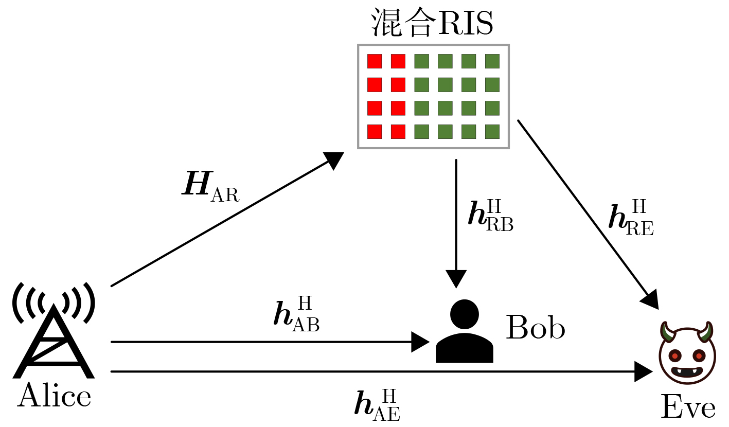
摘要: 针对可重构智能表面(Reconfigurable Intelligent Reflecting Surface, RIS)辅助的物理层安全通信，该文设计了基于混合有源-无源RIS和人工噪声(Artificial Noise, AN)辅助的安全传输方案。考虑基站和RIS的功率约束以及RIS无源反射元件的反射系数恒模约束，以最大化系统安全传输速率为目标，构建基站发射波束成形、AN波束向量、RIS反射系数矩阵联合优化问题。使用交替优化(Alternating Optimization, AO)、权值最小均方误差(Weighted Minimum Mean Square Error, WMMSE)和半定松弛(Semi-definite Relaxation, SDR)算法，求解所构建的变量高度耦合的非凸优化问题。仿真结果表明，混合RIS辅助安全传输方案，能够有效提高系统的安全速率，与无源RIS相比，能够有效克服“双衰落”效应导致的安全速率降低，与有源RIS相比，具有更高的能量效率。
- 可重构智能表面 /
- 混合有源-无源RIS /
- 物理层安全 /
- 人工噪声 /
- 交替优化 /
- 半定松弛
Abstract: A hybrid active-passive Reconfigurable Intelligent reflecting Surface (RIS) and Artificial Noise (AN) based transmission scheme is proposed for the secret communication of the RIS assisted wireless communication system. Aiming at maximizing the secrecy rate, a joint optimization problem over the transmit beamforming and AN vector of the base station and the reflecting coefficient matrix of the RIS is formulated. Then, the Alternating Optimization (AO) method, the weighted Minimum Mean Square Error (MMSE) algorithm and the semi-definite relaxation algorithm are proposed to solve this non-convex optimization problem with highly-coupled variables. The simulation results show that the proposed hybrid RIS and AN based scheme can efficiently improve the secrecy rate of the considered system and overcome the secrecy rate decrease due to the "double fading" effect of the passive RIS. Compared with the full active RIS, the proposed scheme achieves higher energy efficiency.
- Reconfigurable Intelligent Reflecting Surface /
- Hybrid active-passive RIS /
- Physical layer security /
- Artificial noise /
- Alternating optimization /
- Semi-definite relaxation

HTML全文

图 1 系统模型

下载: 全尺寸图片幻灯片

图 2 仿真系统模型坐标图

下载: 全尺寸图片幻灯片

图 3 收敛性能

下载: 全尺寸图片幻灯片

图 4 不同方案中安全速率与功率之间的关系

下载: 全尺寸图片幻灯片

图 5 不同方案中安全速率与距离位置的关系

下载: 全尺寸图片幻灯片

图 6 安全速率与混合RIS中有源元件个数的关系

下载: 全尺寸图片幻灯片

1 交替优化求解算法

1：Initialize
2：给定初始可行解$ {\boldsymbol{w}}^{0}、{\boldsymbol{v}}^{0}、{\boldsymbol{\varPhi}}^{\text{0}} $，设置迭代次数$ i $=0、收敛精度$ \delta $、初始辅助变量$ {{b}}_{\text{1}}^{\text{0}}=1、{{b}}_{\text{2}}^{\text{0}}=1，{\text{R}}^{0}=f\left({\boldsymbol{w}}^{0}，{\boldsymbol{v}}^{0}，{\boldsymbol{\varPhi}}^{\text{0}}\right) $
3：repeat
4：　给定$ {{\boldsymbol{\varPhi}}}^{i} $, $ {{b}}_{\text{1}}^{i} $，$ {{b}}_{\text{2}}^{i} $，根据3.2节所述方法求解问题(P2-2)，并对得出的解进行处理，从而更新$ {\boldsymbol{w}}^{i+1}、{\boldsymbol{v}}^{i+1} $
5：　给定$ {\boldsymbol{w}}^{i+1}，{\boldsymbol{v}}^{i+1} $, $ {{b}}_{\text{1}}^{i} $, $ {{b}}_{\text{2}}^{\mathrm{i}} $根据3.3节所述方法求解问题(P3-2)，对其解进行高斯随机化，得到近似解，进而更新$ {\boldsymbol{\varPhi}}^{i+1} $
6：　给定$ {\boldsymbol{w}}^{i+1}，{\boldsymbol{v}}^{i+1} $，$ {\boldsymbol{\varPhi}}^{i+1} $，根据3.4节所述方法更新辅助变量$ {{b}}_{\text{1}}^{i+1} $，$ {{b}}_{\text{2}}^{i+1} $
7：　$ {{R}}^{i+1}=f\left({\boldsymbol{w}}^{i+1}，{\boldsymbol{v}}^{i+1}，{\boldsymbol{\varPhi}}^{i+1}\right) $
8：　$ i=i+1 $
9：until $ \dfrac{{{R}}^{\boldsymbol{i}}-{{R}}^{\boldsymbol{i}-1}}{{{R}}^{\boldsymbol{i}}} < \delta $

下载: 导出CSV

参考文献(27)

[1]	WU Qingqing and ZHANG Rui. Intelligent reflecting surface enhanced wireless network via joint active and passive beamforming[J]. IEEE Transactions on Wireless Communications, 2019, 18(11): 5394–5409. doi: 10.1109/TWC.2019.2936025.
[2]	WU Qingqing and ZHANG Rui. Towards smart and reconfigurable environment: Intelligent reflecting surface aided wireless network[J]. IEEE Communications Magazine, 2020, 58(1): 106–112. doi: 10.1109/MCOM.001.1900107.
[3]	DONG Lun, HAN Zhu, PETROPULU A P, et al. Improving wireless physical layer security via cooperating relays[J]. IEEE Transactions on Signal Processing, 2010, 58(3): 1875–1888. doi: 10.1109/TSP.2009.2038412.
[4]	BLOCH M, HAYASHI M, and THANGARAJ A. Error-control coding for physical-layer secrecy[J]. Proceedings of the IEEE, 2015, 103(10): 1725–1746. doi: 10.1109/JPROC.2015.2463678.
[5]	FANG Sisai, CHEN Gaojie, ABDULLAH Z, et al. Intelligent Omni surface-assisted secure MIMO communication networks with artificial noise[J]. IEEE Communications Letters, 2022, 26(6): 1231–1235. doi: 10.1109/LCOMM.2022.3159575.
[6]	CUI Miao, ZHANG Guangchi, and ZHANG Rui. Secure wireless communication via intelligent reflecting surface[J]. IEEE Wireless Communications Letters, 2019, 8(5): 1410–1414. doi: 10.1109/LWC.2019.2919685.
[7]	CHEN Siyu, JI Yancheng, JIANG Yan, et al. Optimal RIS allocations for PLS with uncertain jammer and eavesdropper[J]. IEEE Transactions on Consumer Electronics, 2023, 69(4): 927–936. doi: 10.1109/TCE.2023.3292842.
[8]	ZHANG Zhe, ZHANG Chensi, JIANG Chengjun, et al. Improving physical layer security for reconfigurable intelligent surface aided NOMA 6G networks[J]. IEEE Transactions on Vehicular Technology, 2021, 70(5): 4451–4463. doi: 10.1109/TVT.2021.3068774.
[9]	YOU Li, XIONG Jiayuan, NG D W K, et al. Energy efficiency and spectral efficiency tradeoff in RIS-aided multiuser MIMO uplink transmission[J]. IEEE Transactions on Signal Processing, 2021, 69: 1407–1421. doi: 10.1109/TSP.2020.3047474.
[10]	LI Guyue, HU Lei, STAAT P, et al. Reconfigurable intelligent surface for physical layer key generation: Constructive or destructive?[J]. IEEE Wireless Communications, 2022, 29(4): 146–153. doi: 10.1109/MWC.007.2100545.
[11]	LI Guyue, SUN Chen, XU Wei, et al. On maximizing the sum secret key rate for reconfigurable intelligent surface-assisted multiuser systems[J]. IEEE Transactions on Information Forensics and Security, 2022, 17: 211–225. doi: 10.1109/TIFS.2021.3138612.
[12]	LV Weigang, BAI Jiale, YAN Qingli, et al. RIS-assisted green secure communications: Active RIS or passive RIS?[J]. IEEE Wireless Communications Letters, 2023, 12(2): 237–241. doi: 10.1109/LWC.2022.3221609.
[13]	LONG Ruizhe, LIANG Yingchang, PEI Yiyang, et al. Active reconfigurable intelligent surface-aided wireless communications[J]. IEEE Transactions on Wireless Communications, 2021, 20(8): 4962–4975. doi: 10.1109/TWC.2021.3064024.
[14]	KHOSHAFA M H, NGATCHED T M N, AHMED M H, et al. Active reconfigurable intelligent surfaces-aided wireless communication system[J]. IEEE Communications Letters, 2021, 25(11): 3699–3703. doi: 10.1109/LCOMM.2021.3110714.
[15]	DONG Limeng, WANG Huiming, and BAI Jiale. Active reconfigurable intelligent surface aided secure transmission[J]. IEEE Transactions on Vehicular Technology, 2022, 71(2): 2181–2186. doi: 10.1109/TVT.2021.3135498.
[16]	DONG Limeng and YAN Wanyu. Active reconfigurable intelligent surface (RIS) aided secure wireless transmission under a shared power source between transmitter and RIS[C]. 2022 14th International Conference on Wireless Communications and Signal Processing (WCSP), Nanjing, China, 2022: 996–1000. doi: 10.1109/WCSP55476.2022.10039260.
[17]	ZHU Qi, LI Ming, LIU Rang, et al. Joint transceiver beamforming and reflecting design for active RIS-aided ISAC systems[J]. IEEE Transactions on Vehicular Technology, 2023, 72(7): 9636–9640. doi: 10.1109/TVT.2023.3249752.
[18]	YANG Songjie, LYU Wanting, XIU Yue, et al. Active 3D double-RIS-aided multi-user communications: Two-timescale-based separate channel estimation via Bayesian learning[J]. IEEE Transactions on Communications, 2023, 71(6): 3605–3620. doi: 10.1109/TCOMM.2023.3265115.
[19]	NGUYEN N T, VU Q D, LEE K, et al. Hybrid relay-reflecting intelligent surface-assisted wireless communications[J]. IEEE Transactions on Vehicular Technology, 2022, 71(6): 6228–6244. doi: 10.1109/TVT.2022.3158686.
[20]	NGUYEN N T, NGUYEN V D, WU Qingqing, et al. Hybrid active-passive reconfigurable intelligent surface-assisted multi-user MISO systems[C]. 2022 IEEE 23rd International Workshop on Signal Processing Advances in Wireless Communication (SPAWC), Oulu, Finland, 2022: 1–5. doi: 10.1109/SPAWC51304.2022.9833956.
[21]	SCHROEDER R, HE Jiguang, and JUNTTI M. Passive RIS vs. hybrid RIS: A comparative study on channel estimation[C]. 2021 IEEE 93rd Vehicular Technology Conference (VTC2021-Spring), Helsinki, Finland, 2021: 1–7. doi: 10.1109/VTC2021-Spring51267.2021.9448802.
[22]	SCHROEDER R, HE Jiguang, BRANTE G, et al. Two-stage channel estimation for hybrid RIS assisted MIMO systems[J]. IEEE Transactions on Communications, 2022, 70(7): 4793–4806. doi: 10.1109/TCOMM.2022.3176654.
[23]	NGO K H, NGUYEN N T, DINH T Q, et al. Low-latency and secure computation offloading assisted by hybrid relay-reflecting intelligent surface[C]. 2021 International Conference on Advanced Technologies for Communications (ATC), Ho Chi Minh City, Vietnam, 2021: 306–311. doi: 10.1109/ATC52653.2021.9598322.
[24]	NGUYEN N T, VU Q D, LEE K, et al. Spectral efficiency optimization for hybrid relay-reflecting intelligent surface[C]. 2021 IEEE International Conference on Communications Workshops (ICC Workshops), Montreal, Canada, 2021: 1–6. doi: 10.1109/ICCWorkshops50388.2021.9473487.
[25]	SHI Qingjiang, XU Weiqiang, WU Jinsong, et al. Secure beamforming for MIMO broadcasting with wireless information and power transfer[J]. IEEE Transactions on Wireless Communications, 2015, 14(5): 2841–2853. doi: 10.1109/TWC.2015.2395414.
[26]	LUO Zhiquan, MA W K, SO A M C, et al. Semidefinite relaxation of quadratic optimization problems[J]. IEEE Signal Processing Magazine, 2010, 27(3): 20–34. doi: 10.1109/MSP.2010.936019.
[27]	DONG Limeng and WANG Huiming. Enhancing secure MIMO transmission via intelligent reflecting surface[J]. IEEE Transactions on Wireless Communications, 2020, 19(11): 7543–7556. doi: 10.1109/TWC.2020.3012721.